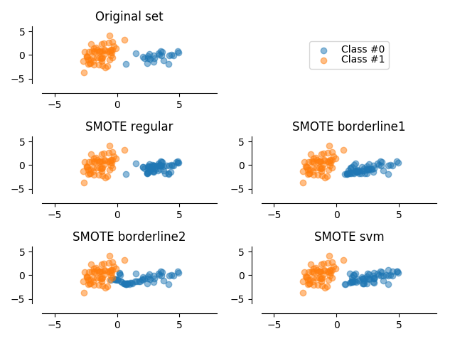
SMOTE¶

An illustration of the SMOTE method and its variant.
# Authors: Fernando Nogueira
#          Christos Aridas
#          Guillaume Lemaitre <g.lemaitre58@gmail.com>
# License: MIT

import matplotlib.pyplot as plt
from sklearn.datasets import make_classification
from sklearn.decomposition import PCA

from imblearn.over_sampling import SMOTE

print(__doc__)


def plot_resampling(ax, X, y, title):
    c0 = ax.scatter(X[y == 0, 0], X[y == 0, 1], label="Class #0", alpha=0.5)
    c1 = ax.scatter(X[y == 1, 0], X[y == 1, 1], label="Class #1", alpha=0.5)
    ax.set_title(title)
    ax.spines['top'].set_visible(False)
    ax.spines['right'].set_visible(False)
    ax.get_xaxis().tick_bottom()
    ax.get_yaxis().tick_left()
    ax.spines['left'].set_position(('outward', 10))
    ax.spines['bottom'].set_position(('outward', 10))
    ax.set_xlim([-6, 8])
    ax.set_ylim([-6, 6])

    return c0, c1


# Generate the dataset
X, y = make_classification(n_classes=2, class_sep=2, weights=[0.3, 0.7],
                           n_informative=3, n_redundant=1, flip_y=0,
                           n_features=20, n_clusters_per_class=1,
                           n_samples=80, random_state=10)

# Instanciate a PCA object for the sake of easy visualisation
pca = PCA(n_components=2)
# Fit and transform x to visualise inside a 2D feature space
X_vis = pca.fit_transform(X)

# Apply regular SMOTE
kind = ['regular', 'borderline1', 'borderline2', 'svm']
sm = [SMOTE(kind=k) for k in kind]
X_resampled = []
y_resampled = []
X_res_vis = []
for method in sm:
    X_res, y_res = method.fit_sample(X, y)
    X_resampled.append(X_res)
    y_resampled.append(y_res)
    X_res_vis.append(pca.transform(X_res))

# Two subplots, unpack the axes array immediately
f, ((ax1, ax2), (ax3, ax4), (ax5, ax6)) = plt.subplots(3, 2)
# Remove axis for second plot
ax2.axis('off')
ax_res = [ax3, ax4, ax5, ax6]

c0, c1 = plot_resampling(ax1, X_vis, y, 'Original set')
for i in range(len(kind)):
    plot_resampling(ax_res[i], X_res_vis[i], y_resampled[i],
                    'SMOTE {}'.format(kind[i]))

ax2.legend((c0, c1), ('Class #0', 'Class #1'), loc='center',
           ncol=1, labelspacing=0.)
plt.tight_layout()
plt.show()
Total running time of the script: ( 0 minutes 0.805 seconds)
Generated by Sphinx-Gallery