Beyond linear separations#
This notebook shows how preprocessing makes linear models flexible enough to fit data with non-linear relationships between features and targets.
# When using JupyterLite, uncomment and install the `skrub` package.
%pip install skrub
import matplotlib.pyplot as plt
import skrub

skrub.patch_display()  # makes nice display for pandas tables
/home/runner/work/traces-sklearn/traces-sklearn/.pixi/envs/docs/bin/python: No module named pip
Note: you may need to restart the kernel to use updated packages.
Limitation of linear separation#
We create a complex classification toy dataset where a linear model will likely fail. Let’s generate the dataset and plot it.
import numpy as np
import pandas as pd
from sklearn.datasets import make_moons

feature_names = ["Feature #0", "Feature #1"]
target_name = "class"

X, y = make_moons(n_samples=100, noise=0.13, random_state=42)

# Store both data and target in a dataframe to ease plotting
moons = pd.DataFrame(
    np.concatenate([X, y[:, np.newaxis]], axis=1), columns=feature_names + [target_name]
)
moons[target_name] = moons[target_name].astype("category")
X, y = moons[feature_names], moons[target_name]
moons.plot.scatter(
    x=feature_names[0],
    y=feature_names[1],
    c=y,
    s=50,
    edgecolor="black",
)
plt.show()
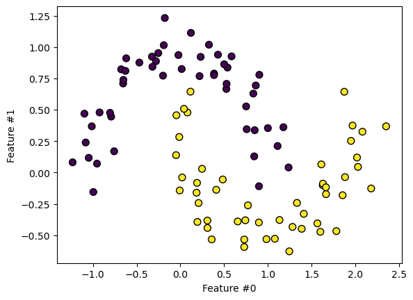
Looking at the dataset, we see that a linear separation cannot effectively discriminate between the classes.
EXERCISE
Fit a
LogisticRegressionmodel on the dataset.Use
sklearn.inspection.DecisionBoundaryDisplayto draw the decision boundary of the model.
# Write your code here.
EXERCISE
Fit a
LogisticRegressionmodel on the dataset but add asklearn.preprocessing.PolynomialFeaturestransformer.Use
sklearn.inspection.DecisionBoundaryDisplayto draw the decision boundary of the model.
# Write your code here.
What about SVM?#
Support Vector Machines (SVM) offer another family of linear algorithms. SVMs use a different training approach than logistic regression. The model finds a hyperplane that maximizes the margin to the closest points.
from sklearn.pipeline import Pipeline
from sklearn.preprocessing import StandardScaler
from sklearn.svm import LinearSVC

model = Pipeline([("scaler", StandardScaler()), ("svc", LinearSVC())])
model.fit(X, y)
Pipeline(steps=[('scaler', StandardScaler()), ('svc', LinearSVC())])In a Jupyter environment, please rerun this cell to show the HTML representation or trust the notebook. On GitHub, the HTML representation is unable to render, please try loading this page with nbviewer.org.
Pipeline(steps=[('scaler', StandardScaler()), ('svc', LinearSVC())])StandardScaler()
LinearSVC()
from sklearn.inspection import DecisionBoundaryDisplay

display = DecisionBoundaryDisplay.from_estimator(model, X, cmap=plt.cm.viridis)
moons.plot.scatter(
    x=feature_names[0], y=feature_names[1], c=y, s=50, edgecolor="black", ax=display.ax_
)
plt.show()
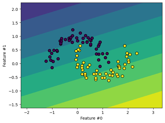
SVMs become non-linear through the “kernel trick”. This projects data into a higher
dimensional space without explicitly building the kernel, only computing dot products.
The SVC class enables kernel use. We use a polynomial kernel to create something
similar to the previous pipeline with PolynomialFeatures.
from sklearn.svm import SVC

model = Pipeline([("scaler", StandardScaler()), ("svc", SVC(kernel="poly", degree=3))])
model.fit(X, y)
Pipeline(steps=[('scaler', StandardScaler()), ('svc', SVC(kernel='poly'))])In a Jupyter environment, please rerun this cell to show the HTML representation or trust the notebook. On GitHub, the HTML representation is unable to render, please try loading this page with nbviewer.org.
Pipeline(steps=[('scaler', StandardScaler()), ('svc', SVC(kernel='poly'))])StandardScaler()
SVC(kernel='poly')
display = DecisionBoundaryDisplay.from_estimator(model, X, cmap=plt.cm.viridis)
moons.plot.scatter(
    x=feature_names[0], y=feature_names[1], c=y, s=50, edgecolor="black", ax=display.ax_
)
plt.show()
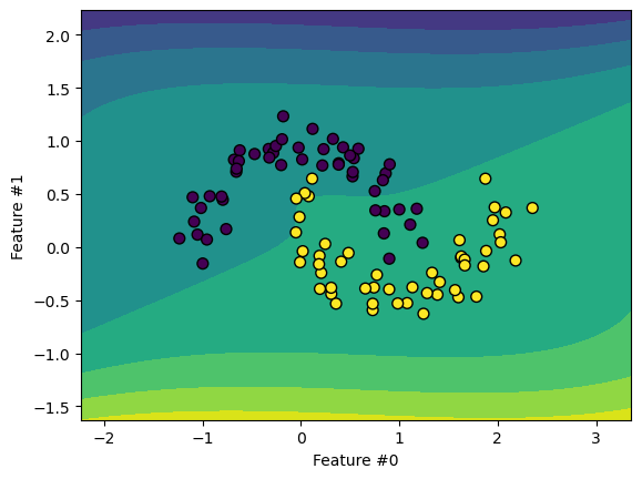
We can also use other kernel types, like the Radial Basis Function (RBF).
from sklearn.svm import SVC

model = Pipeline([("scaler", StandardScaler()), ("svc", SVC(kernel="rbf"))])
model.fit(X, y)
Pipeline(steps=[('scaler', StandardScaler()), ('svc', SVC())])In a Jupyter environment, please rerun this cell to show the HTML representation or trust the notebook. On GitHub, the HTML representation is unable to render, please try loading this page with nbviewer.org.
Pipeline(steps=[('scaler', StandardScaler()), ('svc', SVC())])StandardScaler()
SVC()
display = DecisionBoundaryDisplay.from_estimator(model, X, cmap=plt.cm.viridis)
moons.plot.scatter(
    x=feature_names[0], y=feature_names[1], c=y, s=50, edgecolor="black", ax=display.ax_
)
plt.show()
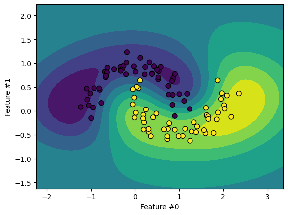
Note that SVMs do not scale well with large datasets. Sometimes it works better to
approximate the kernel explicitly with a transformer like Nystroem.
from sklearn.kernel_approximation import Nystroem
from sklearn.linear_model import LogisticRegression

model = Pipeline(
    [("nystroem", Nystroem()), ("logistic_regression", LogisticRegression())]
)
model.fit(X, y)
Pipeline(steps=[('nystroem', Nystroem()),
                ('logistic_regression', LogisticRegression())])
In a Jupyter environment, please rerun this cell to show the HTML representation or trust the notebook. On GitHub, the HTML representation is unable to render, please try loading this page with nbviewer.org.
Pipeline(steps=[('nystroem', Nystroem()),
('logistic_regression', LogisticRegression())])Nystroem()
LogisticRegression()
display = DecisionBoundaryDisplay.from_estimator(model, X, cmap=plt.cm.viridis)
moons.plot.scatter(
    x=feature_names[0], y=feature_names[1], c=y, s=50, edgecolor="black", ax=display.ax_
)
plt.show()
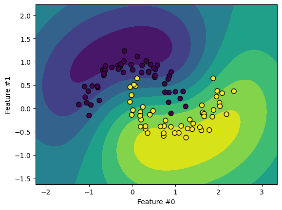
The decision boundary looks similar to an SVM with an RBF kernel. Let’s demonstrate the scaling limitations of SVM classifiers.
data = pd.read_csv("../datasets/adult-census-numeric-all.csv")
data.head()
Processing column 1 / 6
Processing column 2 / 6
Processing column 3 / 6
Processing column 4 / 6
Processing column 5 / 6
Processing column 6 / 6
| age | education-num | capital-gain | capital-loss | hours-per-week | class | |
|---|---|---|---|---|---|---|
| 0 | 25 | 7 | 0 | 0 | 40 | <=50K |
| 1 | 38 | 9 | 0 | 0 | 50 | <=50K |
| 2 | 28 | 12 | 0 | 0 | 40 | >50K |
| 3 | 44 | 10 | 7688 | 0 | 40 | >50K |
| 4 | 18 | 10 | 0 | 0 | 30 | <=50K |
age
Int64DType- Null values
- 0 (0.0%)
- Unique values
- 5 (100.0%)
- Mean ± Std
- 30.6 ± 10.4
- Median ± IQR
- 28 ± 13
- Min | Max
- 18 | 44
education-num
Int64DType- Null values
- 0 (0.0%)
- Unique values
- 4 (80.0%)
- Mean ± Std
- 9.60 ± 1.82
- Median ± IQR
- 10 ± 1
- Min | Max
- 7 | 12
capital-gain
Int64DType- Null values
- 0 (0.0%)
- Unique values
- 2 (40.0%)
- Mean ± Std
- 1.54e+03 ± 3.44e+03
- Median ± IQR
- 0 ± 0
- Min | Max
- 0 | 7,688
capital-loss
Int64DType- Null values
- 0 (0.0%)
hours-per-week
Int64DType- Null values
- 0 (0.0%)
- Unique values
- 3 (60.0%)
- Mean ± Std
- 40.0 ± 7.07
- Median ± IQR
- 40 ± 0
- Min | Max
- 30 | 50
class
ObjectDType- Null values
- 0 (0.0%)
- Unique values
- 2 (40.0%)
Most frequent values
No columns match the selected filter: . You can change the column filter in the dropdown menu above.
| Column | Column name | dtype | Null values | Unique values | Mean | Std | Min | Median | Max |
|---|---|---|---|---|---|---|---|---|---|
| 0 | age | Int64DType | 0 (0.0%) | 5 (100.0%) | 30.6 | 10.4 | 18 | 28 | 44 |
| 1 | education-num | Int64DType | 0 (0.0%) | 4 (80.0%) | 9.60 | 1.82 | 7 | 10 | 12 |
| 2 | capital-gain | Int64DType | 0 (0.0%) | 2 (40.0%) | 1.54e+03 | 3.44e+03 | 0 | 0 | 7,688 |
| 3 | capital-loss | Int64DType | 0 (0.0%) | 1 (20.0%) | 0.00 | 0.00 | |||
| 4 | hours-per-week | Int64DType | 0 (0.0%) | 3 (60.0%) | 40.0 | 7.07 | 30 | 40 | 50 |
| 5 | class | ObjectDType | 0 (0.0%) | 2 (40.0%) |
No columns match the selected filter: . You can change the column filter in the dropdown menu above.
age
Int64DType- Null values
- 0 (0.0%)
- Unique values
- 5 (100.0%)
- Mean ± Std
- 30.6 ± 10.4
- Median ± IQR
- 28 ± 13
- Min | Max
- 18 | 44
education-num
Int64DType- Null values
- 0 (0.0%)
- Unique values
- 4 (80.0%)
- Mean ± Std
- 9.60 ± 1.82
- Median ± IQR
- 10 ± 1
- Min | Max
- 7 | 12
capital-gain
Int64DType- Null values
- 0 (0.0%)
- Unique values
- 2 (40.0%)
- Mean ± Std
- 1.54e+03 ± 3.44e+03
- Median ± IQR
- 0 ± 0
- Min | Max
- 0 | 7,688
capital-loss
Int64DType- Null values
- 0 (0.0%)
hours-per-week
Int64DType- Null values
- 0 (0.0%)
- Unique values
- 3 (60.0%)
- Mean ± Std
- 40.0 ± 7.07
- Median ± IQR
- 40 ± 0
- Min | Max
- 30 | 50
class
ObjectDType- Null values
- 0 (0.0%)
- Unique values
- 2 (40.0%)
Most frequent values
No columns match the selected filter: . You can change the column filter in the dropdown menu above.
| Column 1 | Column 2 | Cramér's V |
|---|---|---|
| age | capital-gain | 1.00 |
| age | education-num | 1.00 |
| age | class | 1.00 |
| age | hours-per-week | 1.00 |
| education-num | hours-per-week | 0.816 |
| education-num | class | 0.764 |
| hours-per-week | class | 0.667 |
| capital-gain | class | 0.612 |
| education-num | capital-gain | 0.612 |
| capital-gain | hours-per-week | 0.408 |
| capital-loss | class | 0.00 |
| capital-gain | capital-loss | 0.00 |
| capital-loss | hours-per-week | 0.00 |
| education-num | capital-loss | 0.00 |
| age | capital-loss | 0.00 |
Please enable javascript
The skrub table reports need javascript to display correctly. If you are displaying a report in a Jupyter notebook and you see this message, you may need to re-execute the cell or to trust the notebook (button on the top right or "File > Trust notebook").
target_name = "class"
X = data.drop(columns=target_name)
y = data[target_name]
X.shape
(48842, 5)
The dataset contains almost 50,000 samples - quite large for an SVM model.
EXERCISE
Split the dataset into training and testing sets.
Create a model with an RBF kernel SVM. Time how long it takes to fit.
Repeat with a model using Nystroem kernel approximation and logistic regression.
Compare the test scores of both models.
# Write your code here.