Boosted trees

This notebook presents a second family of ensemble methods known as boosting. We first give an intuitive example of how boosting works, followed by an introduction to gradient boosting decision tree models.

Introduction to boosting

We start with an intuitive explanation of the boosting principle. In the previous notebook, we saw that bagging creates several datasets with small variations using bootstrapping. An estimator trains on each dataset and aggregates the different results. In boosting, the paradigm differs: the estimators train on the same dataset. To combine them, each estimator corrects the error of all previous estimators. This creates a sequence of estimators instead of independent ones.

Let’s examine an example on a classification dataset.

# When using JupyterLite, uncomment and install the `skrub` package.
%pip install skrub
import matplotlib.pyplot as plt
import skrub

skrub.patch_display()  # makes nice display for pandas tables

/home/runner/work/traces-sklearn/traces-sklearn/.pixi/envs/docs/bin/python: No module named pip

Note: you may need to restart the kernel to use updated packages.

import pandas as pd

data = pd.read_csv("../datasets/penguins_classification.csv")
data["Species"] = data["Species"].astype("category")
X, y = data[["Culmen Length (mm)", "Culmen Depth (mm)"]], data["Species"]

_, ax = plt.subplots(figsize=(8, 6))
data.plot.scatter(
    x="Culmen Length (mm)",
    y="Culmen Depth (mm)",
    c="Species",
    edgecolor="black",
    s=80,
    ax=ax,
)
plt.show()

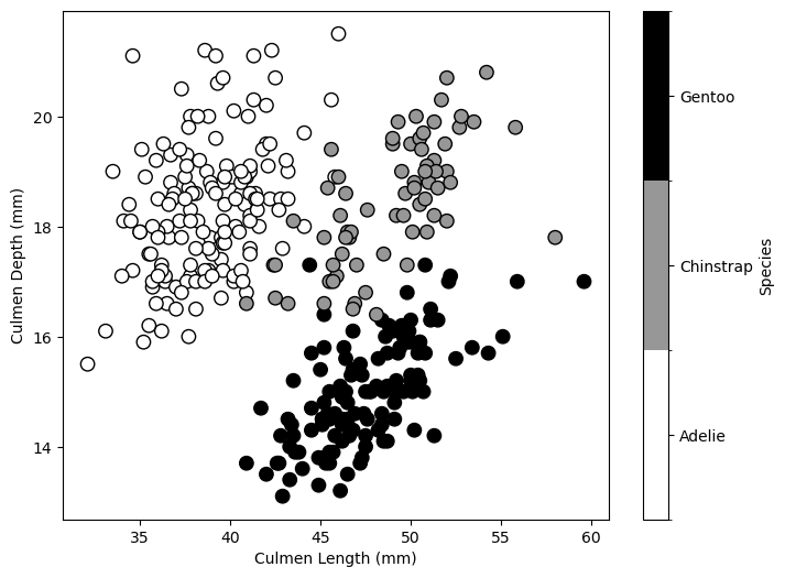
In this dataset, we distinguish three penguin species based on their culmen depth and length. We start by training a shallow decision tree classifier.

from sklearn.tree import DecisionTreeClassifier

tree = DecisionTreeClassifier(max_depth=2, random_state=0)
tree.fit(X, y)

DecisionTreeClassifier(max_depth=2, random_state=0)

In a Jupyter environment, please rerun this cell to show the HTML representation or trust the notebook.
On GitHub, the HTML representation is unable to render, please try loading this page with nbviewer.org.

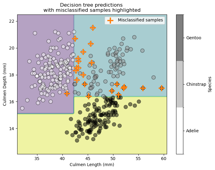
We check the statistical performance of our model qualitatively by examining the decision boundary and highlighting misclassified samples.

import numpy as np

target_predicted = tree.predict(X)
mask_misclassified = y != target_predicted

from sklearn.inspection import DecisionBoundaryDisplay

_, ax = plt.subplots(figsize=(8, 6))

display = DecisionBoundaryDisplay.from_estimator(
    tree, X, response_method="predict", cmap=plt.cm.viridis, alpha=0.4, ax=ax
)

data.plot.scatter(
    x="Culmen Length (mm)",
    y="Culmen Depth (mm)",
    c="Species",
    s=80,
    edgecolor="black",
    alpha=0.5,
    ax=ax,
)

data[mask_misclassified].plot.scatter(
    x="Culmen Length (mm)",
    y="Culmen Depth (mm)",
    s=200,
    marker="+",
    color="tab:orange",
    linewidth=3,
    ax=ax,
    label="Misclassified samples",
)
ax.legend()
ax.set_title("Decision tree predictions \nwith misclassified samples highlighted")
plt.show()

Our decision tree makes several errors for some Gentoo and Adelie samples. Next, we train a new decision tree that focuses only on the misclassified samples. Scikit-learn’s fit method includes a sample_weight parameter that gives more weight to specific samples. We use this parameter to focus our new decision tree on the misclassified samples.

sample_weight = mask_misclassified.astype(np.float64)

tree = DecisionTreeClassifier(max_depth=2, random_state=0)
tree.fit(X, y, sample_weight=sample_weight)

DecisionTreeClassifier(max_depth=2, random_state=0)

In a Jupyter environment, please rerun this cell to show the HTML representation or trust the notebook.
On GitHub, the HTML representation is unable to render, please try loading this page with nbviewer.org.

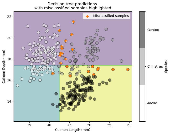
Let’s examine the decision boundary of this newly trained decision tree classifier.

_, ax = plt.subplots(figsize=(8, 6))

display = DecisionBoundaryDisplay.from_estimator(
    tree, X, response_method="predict", cmap=plt.cm.viridis, alpha=0.4, ax=ax
)

data.plot.scatter(
    x="Culmen Length (mm)",
    y="Culmen Depth (mm)",
    c="Species",
    s=80,
    edgecolor="black",
    alpha=0.5,
    ax=ax,
)

data[mask_misclassified].plot.scatter(
    x="Culmen Length (mm)",
    y="Culmen Depth (mm)",
    s=80,
    marker="+",
    color="tab:orange",
    linewidth=3,
    ax=ax,
    label="Misclassified samples",
)
ax.legend()
ax.set_title("Decision tree predictions \nwith misclassified samples highlighted")
plt.show()

target_predicted = tree.predict(X)
mask_new_misclassifier = y != target_predicted
remaining_misclassified_samples_idx = mask_misclassified & mask_new_misclassifier

print(
    f"Number of samples previously misclassified and "
    f"still misclassified: {remaining_misclassified_samples_idx.sum()}"
)

Number of samples previously misclassified and still misclassified: 0

The previously misclassified samples now classify correctly. However, this improvement misclassifies other samples. We could continue training more decision tree classifiers, but we need a way to combine them. One approach weights each classifier based on its accuracy on the full training set.

ensemble_weight = [
    (y.size - mask_misclassified.sum()) / y.size,
    (y.size - mask_new_misclassifier.sum()) / y.size,
]
ensemble_weight

[np.float64(0.935672514619883), np.float64(0.6929824561403509)]

In our example, the first classification achieves good accuracy, so we trust it more than the second classifier. This suggests making a linear combination of the different decision tree classifiers.

This example simplifies an algorithm known as AdaBoostClassifier.

EXERCISE:

1. Train a sklearn.ensemble.AdaBoostClassifier with 3 estimators and a base DecisionTreeClassifier with max_depth=3.

2. Access the fitted attribute estimators_ containing the decision tree classifiers and plot their decision boundaries.

3. Find the weights associated with each decision tree classifier.

# Write your code here.

Gradient Boosting Decision Trees

AdaBoost predictors see less use today. Instead, gradient boosting decision trees demonstrate superior performance.

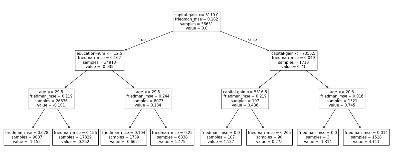
In gradient boosting, each estimator uses a decision tree regressor even for classification. Regression trees provide continuous residuals. Each new estimator trains on the residuals of previous estimators. Parameters control how quickly the model corrects these residuals.

Let’s demonstrate this model on a classification task.

from sklearn.model_selection import train_test_split

data = pd.read_csv("../datasets/adult-census-numeric-all.csv")
X, y = data.drop(columns="class"), data["class"]
X_train, X_test, y_train, y_test = train_test_split(X, y, random_state=0)

from sklearn.ensemble import GradientBoostingClassifier

classifier = GradientBoostingClassifier(n_estimators=5)
classifier.fit(X_train, y_train)

GradientBoostingClassifier(n_estimators=5)

In a Jupyter environment, please rerun this cell to show the HTML representation or trust the notebook.
On GitHub, the HTML representation is unable to render, please try loading this page with nbviewer.org.

classifier.score(X_test, y_test)

0.8056670215379576

Let’s inspect the underlying estimators to confirm our use of decision tree regressors in this classification setting.

classifier.estimators_

array([[DecisionTreeRegressor(criterion='friedman_mse', max_depth=3,
                              random_state=RandomState(MT19937) at 0x7FDE782AF140)],
       [DecisionTreeRegressor(criterion='friedman_mse', max_depth=3,
                              random_state=RandomState(MT19937) at 0x7FDE782AF140)],
       [DecisionTreeRegressor(criterion='friedman_mse', max_depth=3,
                              random_state=RandomState(MT19937) at 0x7FDE782AF140)],
       [DecisionTreeRegressor(criterion='friedman_mse', max_depth=3,
                              random_state=RandomState(MT19937) at 0x7FDE782AF140)],
       [DecisionTreeRegressor(criterion='friedman_mse', max_depth=3,
                              random_state=RandomState(MT19937) at 0x7FDE782AF140)]],
      dtype=object)

from sklearn.tree import plot_tree

_, ax = plt.subplots(figsize=(20, 8))

plot_tree(
    classifier.estimators_[0][0],
    feature_names=X_train.columns,
    ax=ax,
)
plt.show()

Histogram gradient boosting decision trees

EXERCISE: Accelerate gradient boosting

What solutions accelerate the training speed of gradient boosting algorithms?

Short introduction to KBinsDiscretizer

Here’s a trick to accelerate gradient boosting and decision trees in general. Decision trees choose splits from all unique values in a feature. Binning feature values beforehand reduces the number of potential splits to just the bin edges. Since gradient boosting combines several models, the ensemble size compensates for fewer available splits.

Let’s see how to bin a dataset using scikit-learn’s KBinsDiscretizer.

from sklearn.preprocessing import KBinsDiscretizer

discretizer = KBinsDiscretizer(n_bins=10, encode="ordinal", strategy="uniform")
X_trans = discretizer.fit_transform(X)
X_trans

array([[1., 4., 0., 0., 3.],
       [2., 5., 0., 0., 5.],
       [1., 7., 0., 0., 3.],
       ...,
       [5., 5., 0., 0., 3.],
       [0., 5., 0., 0., 1.],
       [4., 5., 1., 0., 3.]])

[len(np.unique(col)) for col in X_trans.T]

[10, 10, 6, 10, 10]

We use 10 bins for each feature.

EXERCISE:

1. Create a pipeline with a KBinsDiscretizer followed by a GradientBoostingClassifier.

2. Compare its training time to a vanilla GradientBoostingClassifier.

# Write your code here.

Scikit-learn provides HistGradientBoostingClassifier, an approximate gradient boosting algorithm similar to lightgbm and xgboost.

import time

from sklearn.ensemble import HistGradientBoostingClassifier

clf = HistGradientBoostingClassifier(max_iter=200, max_bins=10)

start = time.time()
clf.fit(X_train, y_train)
end = time.time()
print(f"Training time: {end - start:.3f} seconds")

Training time: 0.202 seconds

clf.score(X_test, y_test)

0.8091065432806486

Hyperparameters

Gradient boosting couples its parameters, so we must set them together. The key parameters include n_estimators, max_depth, and learning_rate.

The max_depth parameter matters because gradient boosting fits the error of previous trees. Full-grown trees harm performance - the first tree would overfit the data, leaving no residuals for subsequent trees. Trees in gradient boosting work best with low depth (3-8 levels). Weak learners at each step reduce overfitting.

Deeper trees correct residuals faster, requiring fewer learners. Thus, lower max_depth values need more n_estimators.

The learning_rate parameter controls how aggressively trees correct errors. Low learning rates correct residuals for fewer samples. High rates (e.g., 1) correct residuals for all samples. Very low learning rates need more estimators, while high rates risk overfitting like deep trees.

The next chapter covers finding optimal hyperparameter combinations.

The early_stopping parameter helps in histogram gradient boosting. It splits data during fit and uses a validation set to measure improvement from new trees. If new estimators stop improving performance, fitting stops. Let’s see this in action:

model = HistGradientBoostingClassifier(early_stopping=True, max_iter=1_000)
model.fit(X_train, y_train)

HistGradientBoostingClassifier(early_stopping=True, max_iter=1000)

In a Jupyter environment, please rerun this cell to show the HTML representation or trust the notebook.
On GitHub, the HTML representation is unable to render, please try loading this page with nbviewer.org.

We requested 1,000 trees - more than needed. Let’s check how many trees the model actually used:

model.n_iter_

127

The gradient boosting stopped after 127 trees, determining additional trees would not improve performance.