Decision trees#
We explore a class of algorithms based on decision trees. Decision trees are extremely intuitive at their core. They encode a series of “if” and “else” choices, similar to how a person makes a decision. The data determines which questions to ask and how to proceed for each answer.
For example, to create a guide for identifying an animal found in nature, you might ask the following series of questions:
Is the animal bigger or smaller than a meter long?
bigger: does the animal have horns?
yes: are the horns longer than ten centimeters?
no: does the animal wear a collar?
smaller: does the animal have two or four legs?
two: does the animal have wings?
four: does the animal have a bushy tail?
And so on. This binary splitting of questions forms the essence of a decision tree.
Tree-based models offer several key benefits. First, they require little preprocessing of the data. They work with variables of different types (continuous and discrete) and remain invariant to feature scaling.
Tree-based models are also “nonparametric”, meaning they do not have a fixed set of parameters to learn. Instead, a tree model becomes more flexible with more data. In other words, the number of free parameters grows with the number of samples and is not fixed like in linear models.
Decision tree for classification#
Let’s get some intuitions on how a decision tree works on a very simple dataset.
# When using JupyterLite, uncomment and install the `skrub` package.
%pip install skrub
import matplotlib.pyplot as plt
import skrub

skrub.patch_display()  # makes nice display for pandas tables
/home/runner/work/traces-sklearn/traces-sklearn/.pixi/envs/docs/bin/python: No module named pip
Note: you may need to restart the kernel to use updated packages.
from sklearn.datasets import make_blobs

X, y = make_blobs(n_samples=100, centers=[[0, 0], [1, 1]], random_state=42)
import numpy as np
import pandas as pd

X = pd.DataFrame(X, columns=["Feature #0", "Feature #1"])
class_names = np.array(["class #0", "class #1"])
y = pd.Series(class_names[y], name="Classes").astype("category")
data = pd.concat([X, y], axis=1)
data.plot.scatter(
    x="Feature #0",
    y="Feature #1",
    c="Classes",
    s=50,
    edgecolor="black",
)
plt.show()
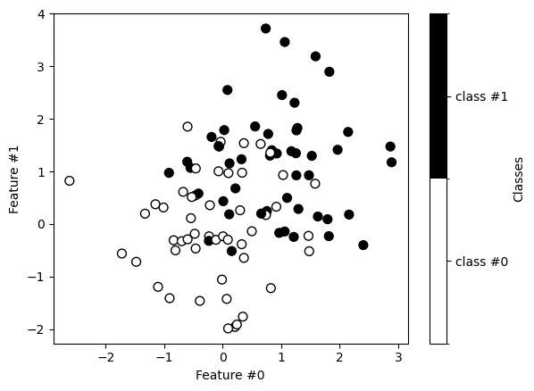
Now, we train a decision tree classifier on this dataset. We first split the data into training and testing sets.
from sklearn.model_selection import train_test_split

data_train, data_test, X_train, X_test, y_train, y_test = train_test_split(
    data, X, y, random_state=42
)
from sklearn.tree import DecisionTreeClassifier

tree = DecisionTreeClassifier(max_depth=1)
tree.fit(X_train, y_train)
pred = tree.predict(X_test)
pred
array(['class #1', 'class #0', 'class #0', 'class #0', 'class #1',
       'class #1', 'class #0', 'class #0', 'class #0', 'class #0',
       'class #0', 'class #1', 'class #0', 'class #0', 'class #0',
       'class #1', 'class #0', 'class #1', 'class #0', 'class #0',
       'class #0', 'class #0', 'class #0', 'class #0', 'class #1'],
      dtype=object)
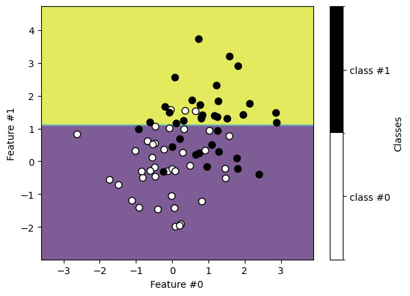
We plot the decision boundaries found using the training data.
from sklearn.inspection import DecisionBoundaryDisplay

display = DecisionBoundaryDisplay.from_estimator(tree, X_train, alpha=0.7)
data_train.plot.scatter(
    x="Feature #0", y="Feature #1", c="Classes", s=50, edgecolor="black", ax=display.ax_
)
plt.show()
Similarly, we get the following classification on the testing set.
display = DecisionBoundaryDisplay.from_estimator(tree, X_test, alpha=0.7)
data_test.plot.scatter(
    x="Feature #0", y="Feature #1", c="Classes", s=50, edgecolor="black", ax=display.ax_
)
plt.show()
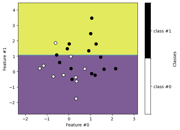
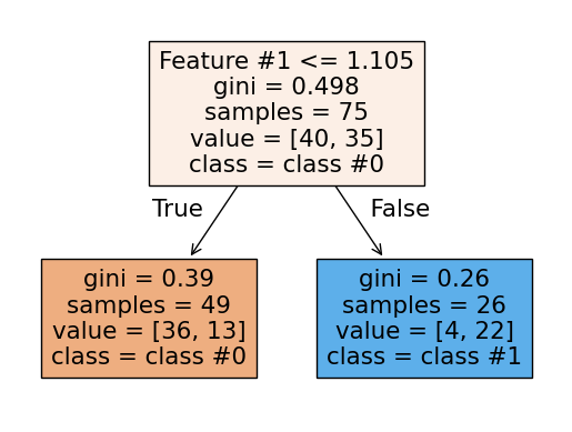
We see that the decision found with a decision tree is a simple binary split.
We can also plot the tree structure.
from sklearn.tree import plot_tree

plot_tree(tree, feature_names=X.columns, class_names=class_names, filled=True)
plt.show()
EXERCISE
Modify the depth of the tree and observe how the partitioning evolves.
What can you conclude about under- and over-fitting of the tree model?
How would you choose the best depth?
Many parameters control the complexity of a tree, but maximum depth is perhaps the easiest to understand. This parameter limits how finely the tree can partition the input space, or how many “if-else” questions it can ask before deciding which class a sample belongs to.
This parameter is crucial to tune for trees and tree-based models. The interactive
plot below shows how underfitting and overfitting look for this model. A
max_depth of 1 clearly underfits the model, while a depth of 7 or 8 clearly
overfits. The maximum possible depth for this dataset is 8, at which point each leaf
contains samples from only a single class. We call these leaves “pure.”
In the interactive plot below, blue and red colors indicate the predicted class for each region. The shade of color indicates the predicted probability for that class (darker = higher probability), while yellow regions indicate equal predicted probability for either class.
Note about partitioning in decision trees#
In this section, we examine in more detail how a tree selects the best partition. First, we use a real dataset instead of synthetic data.
dataset = pd.read_csv("../datasets/penguins.csv")
dataset = dataset.dropna(subset=["Body Mass (g)"])
dataset.head()
Processing column 1 / 17
Processing column 2 / 17
Processing column 3 / 17
Processing column 4 / 17
Processing column 5 / 17
Processing column 6 / 17
Processing column 7 / 17
Processing column 8 / 17
Processing column 9 / 17
Processing column 10 / 17
Processing column 11 / 17
Processing column 12 / 17
Processing column 13 / 17
Processing column 14 / 17
Processing column 15 / 17
Processing column 16 / 17
Processing column 17 / 17
| studyName | Sample Number | Species | Region | Island | Stage | Individual ID | Clutch Completion | Date Egg | Culmen Length (mm) | Culmen Depth (mm) | Flipper Length (mm) | Body Mass (g) | Sex | Delta 15 N (o/oo) | Delta 13 C (o/oo) | Comments | |
|---|---|---|---|---|---|---|---|---|---|---|---|---|---|---|---|---|---|
| 0 | PAL0708 | 1 | Adelie Penguin (Pygoscelis adeliae) | Anvers | Torgersen | Adult, 1 Egg Stage | N1A1 | Yes | 2007-11-11 | 39.1 | 18.7 | 181.0 | 3750.0 | MALE | Not enough blood for isotopes. | ||
| 1 | PAL0708 | 2 | Adelie Penguin (Pygoscelis adeliae) | Anvers | Torgersen | Adult, 1 Egg Stage | N1A2 | Yes | 2007-11-11 | 39.5 | 17.4 | 186.0 | 3800.0 | FEMALE | 8.94956 | -24.69454 | |
| 2 | PAL0708 | 3 | Adelie Penguin (Pygoscelis adeliae) | Anvers | Torgersen | Adult, 1 Egg Stage | N2A1 | Yes | 2007-11-16 | 40.3 | 18.0 | 195.0 | 3250.0 | FEMALE | 8.36821 | -25.33302 | |
| 4 | PAL0708 | 5 | Adelie Penguin (Pygoscelis adeliae) | Anvers | Torgersen | Adult, 1 Egg Stage | N3A1 | Yes | 2007-11-16 | 36.7 | 19.3 | 193.0 | 3450.0 | FEMALE | 8.76651 | -25.32426 | |
| 5 | PAL0708 | 6 | Adelie Penguin (Pygoscelis adeliae) | Anvers | Torgersen | Adult, 1 Egg Stage | N3A2 | Yes | 2007-11-16 | 39.3 | 20.6 | 190.0 | 3650.0 | MALE | 8.66496 | -25.29805 |
studyName
ObjectDType- Null values
- 0 (0.0%)
Sample Number
Int64DType- Null values
- 0 (0.0%)
- Unique values
- 5 (100.0%)
- Mean ± Std
- 3.40 ± 2.07
- Median ± IQR
- 3 ± 3
- Min | Max
- 1 | 6
Species
ObjectDType- Null values
- 0 (0.0%)
Region
ObjectDType- Null values
- 0 (0.0%)
Island
ObjectDType- Null values
- 0 (0.0%)
Stage
ObjectDType- Null values
- 0 (0.0%)
Individual ID
ObjectDType- Null values
- 0 (0.0%)
- Unique values
- 5 (100.0%)
Most frequent values
Clutch Completion
ObjectDType- Null values
- 0 (0.0%)
Date Egg
ObjectDType- Null values
- 0 (0.0%)
- Unique values
- 2 (40.0%)
Most frequent values
Culmen Length (mm)
Float64DType- Null values
- 0 (0.0%)
- Unique values
- 5 (100.0%)
- Mean ± Std
- 39.0 ± 1.35
- Median ± IQR
- 39.3 ± 0.400
- Min | Max
- 36.7 | 40.3
Culmen Depth (mm)
Float64DType- Null values
- 0 (0.0%)
- Unique values
- 5 (100.0%)
- Mean ± Std
- 18.8 ± 1.23
- Median ± IQR
- 18.7 ± 1.30
- Min | Max
- 17.4 | 20.6
Flipper Length (mm)
Float64DType- Null values
- 0 (0.0%)
- Unique values
- 5 (100.0%)
- Mean ± Std
- 189. ± 5.61
- Median ± IQR
- 190. ± 7.00
- Min | Max
- 181. | 195.
Body Mass (g)
Float64DType- Null values
- 0 (0.0%)
- Unique values
- 5 (100.0%)
- Mean ± Std
- 3.58e+03 ± 228.
- Median ± IQR
- 3.65e+03 ± 300.
- Min | Max
- 3.25e+03 | 3.80e+03
Sex
ObjectDType- Null values
- 0 (0.0%)
- Unique values
- 2 (40.0%)
Most frequent values
Delta 15 N (o/oo)
Float64DType- Null values
- 1 (20.0%)
- Unique values
- 4 (80.0%)
- Mean ± Std
- 8.69 ± 0.243
- Median ± IQR
- 8.77 ± 0.102
- Min | Max
- 8.37 | 8.95
Delta 13 C (o/oo)
Float64DType- Null values
- 1 (20.0%)
- Unique values
- 4 (80.0%)
- Mean ± Std
- -25.2 ± 0.312
- Median ± IQR
- -25.3 ± 0.0262
- Min | Max
- -25.3 | -24.7
Comments
ObjectDType- Null values
- 4 (80.0%)
No columns match the selected filter: . You can change the column filter in the dropdown menu above.
| Column | Column name | dtype | Null values | Unique values | Mean | Std | Min | Median | Max |
|---|---|---|---|---|---|---|---|---|---|
| 0 | studyName | ObjectDType | 0 (0.0%) | 1 (20.0%) | |||||
| 1 | Sample Number | Int64DType | 0 (0.0%) | 5 (100.0%) | 3.40 | 2.07 | 1 | 3 | 6 |
| 2 | Species | ObjectDType | 0 (0.0%) | 1 (20.0%) | |||||
| 3 | Region | ObjectDType | 0 (0.0%) | 1 (20.0%) | |||||
| 4 | Island | ObjectDType | 0 (0.0%) | 1 (20.0%) | |||||
| 5 | Stage | ObjectDType | 0 (0.0%) | 1 (20.0%) | |||||
| 6 | Individual ID | ObjectDType | 0 (0.0%) | 5 (100.0%) | |||||
| 7 | Clutch Completion | ObjectDType | 0 (0.0%) | 1 (20.0%) | |||||
| 8 | Date Egg | ObjectDType | 0 (0.0%) | 2 (40.0%) | |||||
| 9 | Culmen Length (mm) | Float64DType | 0 (0.0%) | 5 (100.0%) | 39.0 | 1.35 | 36.7 | 39.3 | 40.3 |
| 10 | Culmen Depth (mm) | Float64DType | 0 (0.0%) | 5 (100.0%) | 18.8 | 1.23 | 17.4 | 18.7 | 20.6 |
| 11 | Flipper Length (mm) | Float64DType | 0 (0.0%) | 5 (100.0%) | 189. | 5.61 | 181. | 190. | 195. |
| 12 | Body Mass (g) | Float64DType | 0 (0.0%) | 5 (100.0%) | 3.58e+03 | 228. | 3.25e+03 | 3.65e+03 | 3.80e+03 |
| 13 | Sex | ObjectDType | 0 (0.0%) | 2 (40.0%) | |||||
| 14 | Delta 15 N (o/oo) | Float64DType | 1 (20.0%) | 4 (80.0%) | 8.69 | 0.243 | 8.37 | 8.77 | 8.95 |
| 15 | Delta 13 C (o/oo) | Float64DType | 1 (20.0%) | 4 (80.0%) | -25.2 | 0.312 | -25.3 | -25.3 | -24.7 |
| 16 | Comments | ObjectDType | 4 (80.0%) | 1 (20.0%) |
No columns match the selected filter: . You can change the column filter in the dropdown menu above.
studyName
ObjectDType- Null values
- 0 (0.0%)
Sample Number
Int64DType- Null values
- 0 (0.0%)
- Unique values
- 5 (100.0%)
- Mean ± Std
- 3.40 ± 2.07
- Median ± IQR
- 3 ± 3
- Min | Max
- 1 | 6
Species
ObjectDType- Null values
- 0 (0.0%)
Region
ObjectDType- Null values
- 0 (0.0%)
Island
ObjectDType- Null values
- 0 (0.0%)
Stage
ObjectDType- Null values
- 0 (0.0%)
Individual ID
ObjectDType- Null values
- 0 (0.0%)
- Unique values
- 5 (100.0%)
Most frequent values
Clutch Completion
ObjectDType- Null values
- 0 (0.0%)
Date Egg
ObjectDType- Null values
- 0 (0.0%)
- Unique values
- 2 (40.0%)
Most frequent values
Culmen Length (mm)
Float64DType- Null values
- 0 (0.0%)
- Unique values
- 5 (100.0%)
- Mean ± Std
- 39.0 ± 1.35
- Median ± IQR
- 39.3 ± 0.400
- Min | Max
- 36.7 | 40.3
Culmen Depth (mm)
Float64DType- Null values
- 0 (0.0%)
- Unique values
- 5 (100.0%)
- Mean ± Std
- 18.8 ± 1.23
- Median ± IQR
- 18.7 ± 1.30
- Min | Max
- 17.4 | 20.6
Flipper Length (mm)
Float64DType- Null values
- 0 (0.0%)
- Unique values
- 5 (100.0%)
- Mean ± Std
- 189. ± 5.61
- Median ± IQR
- 190. ± 7.00
- Min | Max
- 181. | 195.
Body Mass (g)
Float64DType- Null values
- 0 (0.0%)
- Unique values
- 5 (100.0%)
- Mean ± Std
- 3.58e+03 ± 228.
- Median ± IQR
- 3.65e+03 ± 300.
- Min | Max
- 3.25e+03 | 3.80e+03
Sex
ObjectDType- Null values
- 0 (0.0%)
- Unique values
- 2 (40.0%)
Most frequent values
Delta 15 N (o/oo)
Float64DType- Null values
- 1 (20.0%)
- Unique values
- 4 (80.0%)
- Mean ± Std
- 8.69 ± 0.243
- Median ± IQR
- 8.77 ± 0.102
- Min | Max
- 8.37 | 8.95
Delta 13 C (o/oo)
Float64DType- Null values
- 1 (20.0%)
- Unique values
- 4 (80.0%)
- Mean ± Std
- -25.2 ± 0.312
- Median ± IQR
- -25.3 ± 0.0262
- Min | Max
- -25.3 | -24.7
Comments
ObjectDType- Null values
- 4 (80.0%)
No columns match the selected filter: . You can change the column filter in the dropdown menu above.
| Column 1 | Column 2 | Cramér's V |
|---|---|---|
| Delta 13 C (o/oo) | Comments | 1.00 |
| Delta 15 N (o/oo) | Comments | 1.00 |
| Delta 15 N (o/oo) | Delta 13 C (o/oo) | 1.00 |
| Sex | Delta 13 C (o/oo) | 1.00 |
| Body Mass (g) | Comments | 1.00 |
| Sex | Delta 15 N (o/oo) | 1.00 |
| Body Mass (g) | Delta 13 C (o/oo) | 1.00 |
| Body Mass (g) | Delta 15 N (o/oo) | 1.00 |
| Individual ID | Date Egg | 1.00 |
| Body Mass (g) | Sex | 1.00 |
| Flipper Length (mm) | Comments | 1.00 |
| Flipper Length (mm) | Delta 13 C (o/oo) | 1.00 |
| Flipper Length (mm) | Delta 15 N (o/oo) | 1.00 |
| Flipper Length (mm) | Sex | 1.00 |
| Flipper Length (mm) | Body Mass (g) | 1.00 |
| Culmen Depth (mm) | Comments | 1.00 |
| Culmen Depth (mm) | Delta 13 C (o/oo) | 1.00 |
| Culmen Depth (mm) | Delta 15 N (o/oo) | 1.00 |
| Culmen Depth (mm) | Sex | 1.00 |
| Culmen Depth (mm) | Body Mass (g) | 1.00 |
Please enable javascript
The skrub table reports need javascript to display correctly. If you are displaying a report in a Jupyter notebook and you see this message, you may need to re-execute the cell or to trust the notebook (button on the top right or "File > Trust notebook").
We build a decision tree to classify penguin species using their body mass as a feature. To simplify the problem, we focus only on the Adelie and Gentoo species.
# Only select the column of interest
dataset = dataset[["Body Mass (g)", "Species"]]
# Make the species name more readable
dataset["Species"] = dataset["Species"].apply(lambda x: x.split()[0])
# Only select the Adelie and Gentoo penguins
dataset = dataset.set_index("Species").loc[["Adelie", "Gentoo"], :]
# Sort all penguins by their body mass
dataset = dataset.sort_values(by="Body Mass (g)")
# Convert the dataframe (2D) to a series (1D)
dataset = dataset.squeeze()
dataset
Species
Adelie    2850.0
Adelie    2850.0
Adelie    2900.0
Adelie    2900.0
Adelie    2900.0
           ...
Gentoo    5950.0
Gentoo    6000.0
Gentoo    6000.0
Gentoo    6050.0
Gentoo    6300.0
Name: Body Mass (g), Length: 274, dtype: float64
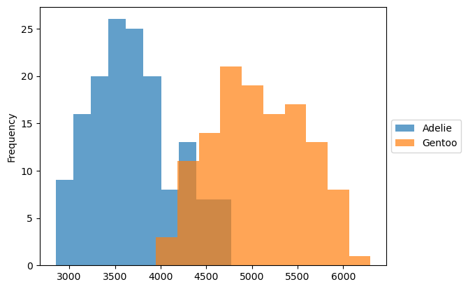
First, we examine the body mass distribution for each species.
_, ax = plt.subplots()
dataset.groupby("Species").plot.hist(ax=ax, alpha=0.7, legend=True)
ax.set_ylabel("Frequency")
ax.legend(loc="center left", bbox_to_anchor=(1, 0.5))
plt.show()
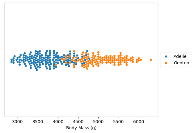
Instead of looking at the distribution, we can look at all samples directly.
%pip install seaborn
import seaborn as sns

ax = sns.swarmplot(x=dataset.values, y=[""] * len(dataset), hue=dataset.index)
ax.set_xlabel(dataset.name)
ax.legend(loc="center left", bbox_to_anchor=(1, 0.5))
plt.show()
/home/runner/work/traces-sklearn/traces-sklearn/.pixi/envs/docs/bin/python: No module named pip
Note: you may need to restart the kernel to use updated packages.
When we build a tree, we want to find splits that partition the data into groups that are as “unmixed” as possible. Let’s make a first completely random split to highlight the principle.
# create a random state so we all get the same results
rng = np.random.default_rng(42)
random_idx = rng.choice(dataset.size)

ax = sns.swarmplot(x=dataset.values, y=[""] * len(dataset), hue=dataset.index)
ax.set_xlabel(dataset.name)
ax.set_title(f"Body mass threshold: {dataset.iloc[random_idx]} grams")
ax.vlines(dataset.iloc[random_idx], -1, 1, color="red", linestyle="--")
ax.legend(loc="center left", bbox_to_anchor=(1, 0.5))
plt.show()
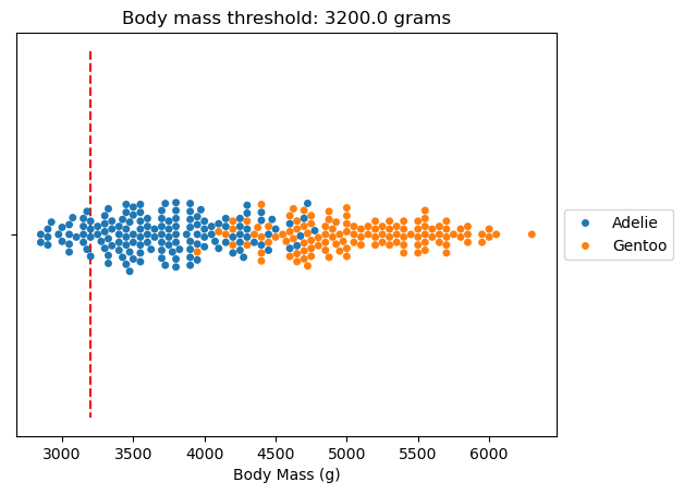
After the split, we want two partitions where samples come from a single class as much as possible and contain as many samples as possible. Decision trees use a criterion to assess split quality. Entropy describes the class mixture in a partition. Let’s compute the entropy for the full dataset and the sets on each side of the split.
from scipy.stats import entropy

dataset.index.value_counts()

parent_entropy = entropy(dataset.index.value_counts(normalize=True))
parent_entropy

left_entropy = entropy(dataset[:random_idx].index.value_counts(normalize=True))
left_entropy

right_entropy = entropy(dataset[random_idx:].index.value_counts(normalize=True))
right_entropy
np.float64(0.6930191750980527)
We assess split quality by combining the entropies. This is called the information gain.
parent_entropy - (left_entropy + right_entropy)
np.float64(-0.005102495972248544)
However, we should normalize the entropies by the number of samples in each set.
def information_gain(labels_parent, labels_left, labels_right):
    # compute the entropies
    entropy_parent = entropy(labels_parent.value_counts(normalize=True))
    entropy_left = entropy(labels_left.value_counts(normalize=True))
    entropy_right = entropy(labels_right.value_counts(normalize=True))

    n_samples_parent = labels_parent.size
    n_samples_left = labels_left.size
    n_samples_right = labels_right.size

    # normalize with the number of samples
    normalized_entropy_left = (n_samples_left / n_samples_parent) * entropy_left
    normalized_entropy_right = (n_samples_right / n_samples_parent) * entropy_right

    return entropy_parent - normalized_entropy_left - normalized_entropy_right


information_gain(dataset.index, dataset[:random_idx].index, dataset[random_idx:].index)
np.float64(0.055599913525391065)
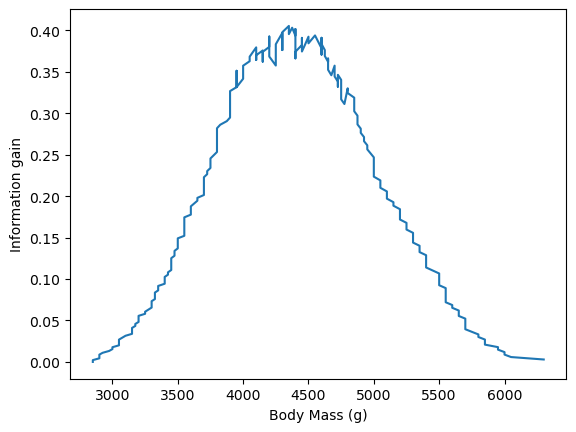
Now we compute the information gain for all possible body mass thresholds.
all_information_gain = pd.Series(
    [
        information_gain(dataset.index, dataset[:idx].index, dataset[idx:].index)
        for idx in range(dataset.size)
    ],
    index=dataset,
)
ax = all_information_gain.plot()
ax.set_ylabel("Information gain")
plt.show()
ax = (all_information_gain * -1).plot(color="red", label="Information gain")
ax = sns.swarmplot(x=dataset.values, y=[""] * len(dataset), hue=dataset.index)
ax.legend(loc="center left", bbox_to_anchor=(1, 0.5))
plt.show()
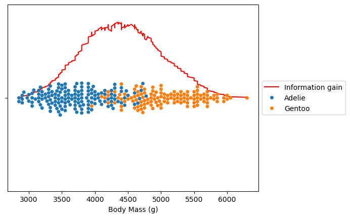
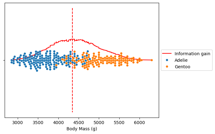
The maximum information gain corresponds to the split that best partitions our data. Let’s check the corresponding body mass threshold.
all_information_gain.idxmax()

ax = (all_information_gain * -1).plot(color="red", label="Information gain")
ax = sns.swarmplot(x=dataset.values, y=[""] * len(dataset), hue=dataset.index)
ax.vlines(all_information_gain.idxmax(), -1, 1, color="red", linestyle="--")
ax.legend(loc="center left", bbox_to_anchor=(1, 0.5))

plt.show()
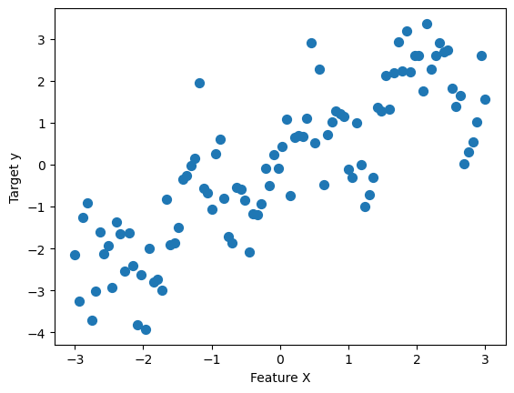
Decision Tree Regression#
rnd = np.random.default_rng(42)
x = np.linspace(-3, 3, 100)
y_no_noise = np.sin(4 * x) + x
y = y_no_noise + rnd.normal(size=len(x))
X = x.reshape(-1, 1)
_, ax = plt.subplots()
ax.scatter(X, y, s=50)
ax.set(xlabel="Feature X", ylabel="Target y")
plt.show()
from sklearn.tree import DecisionTreeRegressor

reg = DecisionTreeRegressor(max_depth=2)
reg.fit(X, y)
DecisionTreeRegressor(max_depth=2)In a Jupyter environment, please rerun this cell to show the HTML representation or trust the notebook.
On GitHub, the HTML representation is unable to render, please try loading this page with nbviewer.org.
DecisionTreeRegressor(max_depth=2)
X_test = np.linspace(-3, 3, 1000).reshape((-1, 1))
y_test = reg.predict(X_test)

_, ax = plt.subplots()
ax.plot(X_test.ravel(), y_test, color="tab:blue", label="prediction")
ax.plot(X.ravel(), y, "C7.", label="training data")
ax.legend(loc="center left", bbox_to_anchor=(1, 0.5))
plt.show()
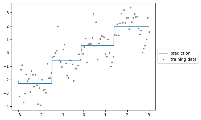
A single decision tree estimates the signal non-parametrically but has some issues. In some regions, the model shows high bias and underfits the data (seen in long flat lines that don’t follow data contours), while in other regions it shows high variance and overfits (seen in narrow spikes influenced by noise in single points).
EXERCISE
Take the above example and repeat the training/testing by changing the tree depth.
What can you conclude?
Other tree hyperparameters#
The max_depth hyperparameter controls overall tree complexity. This parameter works well when a tree is symmetric. However, trees are not guaranteed to be symmetric. In fact, optimal generalization might require some branches to grow deeper than others.
We build a dataset to illustrate this asymmetry. We generate a dataset with 2 subsets: one where the tree should find a clear separation and another where samples from both classes mix. This means a decision tree needs more splits to properly classify samples from the second subset than from the first subset.
from sklearn.datasets import make_blobs

feature_names = ["Feature #0", "Feature #1"]
target_name = "Class"

# Blobs that will be interlaced
X_1, y_1 = make_blobs(n_samples=300, centers=[[0, 0], [-1, -1]], random_state=0)
# Blobs that will be easily separated
X_2, y_2 = make_blobs(n_samples=300, centers=[[3, 6], [7, 0]], random_state=0)

X = np.concatenate([X_1, X_2], axis=0)
y = np.concatenate([y_1, y_2])
data = np.concatenate([X, y[:, np.newaxis]], axis=1)
data = pd.DataFrame(data, columns=feature_names + [target_name])
data[target_name] = data[target_name].astype(np.int64).astype("category")
data
Processing column 1 / 3
Processing column 2 / 3
Processing column 3 / 3
| Feature #0 | Feature #1 | Class | |
|---|---|---|---|
| 0 | 0.9500884175255894 | -0.1513572082976979 | 0 |
| 1 | 1.9559123082506942 | 0.39009332268792646 | 0 |
| 2 | -1.353431748757199 | -2.6164741886510328 | 1 |
| 3 | -0.45553250351734315 | 0.01747915902505673 | 0 |
| 4 | 0.46566243973045984 | -1.5362436862772237 | 0 |
| 595 | 7.453781912635684 | -1.8297404110045314 | 1 |
| 596 | 2.2604370036086867 | 7.543014595406736 | 0 |
| 597 | 4.099659595887113 | 6.655263730722598 | 0 |
| 598 | 7.284279670807215 | 1.7426687806556311 | 1 |
| 599 | 8.078197303714237 | -2.5591846663440965 | 1 |
Feature #0
Float64DType- Null values
- 0 (0.0%)
- Unique values
- 600 (100.0%)
- Mean ± Std
- 2.16 ± 3.26
- Median ± IQR
- 1.71 ± 5.54
- Min | Max
- -3.66 | 9.70
Feature #1
Float64DType- Null values
- 0 (0.0%)
- Unique values
- 600 (100.0%)
- Mean ± Std
- 1.23 ± 3.01
- Median ± IQR
- 0.122 ± 3.26
- Min | Max
- -4.05 | 8.24
Class
CategoricalDtype- Null values
- 0 (0.0%)
- Unique values
- 2 (0.3%)
Most frequent values
No columns match the selected filter: . You can change the column filter in the dropdown menu above.
| Column | Column name | dtype | Null values | Unique values | Mean | Std | Min | Median | Max |
|---|---|---|---|---|---|---|---|---|---|
| 0 | Feature #0 | Float64DType | 0 (0.0%) | 600 (100.0%) | 2.16 | 3.26 | -3.66 | 1.71 | 9.70 |
| 1 | Feature #1 | Float64DType | 0 (0.0%) | 600 (100.0%) | 1.23 | 3.01 | -4.05 | 0.122 | 8.24 |
| 2 | Class | CategoricalDtype | 0 (0.0%) | 2 (0.3%) |
No columns match the selected filter: . You can change the column filter in the dropdown menu above.
Feature #0
Float64DType- Null values
- 0 (0.0%)
- Unique values
- 600 (100.0%)
- Mean ± Std
- 2.16 ± 3.26
- Median ± IQR
- 1.71 ± 5.54
- Min | Max
- -3.66 | 9.70
Feature #1
Float64DType- Null values
- 0 (0.0%)
- Unique values
- 600 (100.0%)
- Mean ± Std
- 1.23 ± 3.01
- Median ± IQR
- 0.122 ± 3.26
- Min | Max
- -4.05 | 8.24
Class
CategoricalDtype- Null values
- 0 (0.0%)
- Unique values
- 2 (0.3%)
Most frequent values
No columns match the selected filter: . You can change the column filter in the dropdown menu above.
| Column 1 | Column 2 | Cramér's V |
|---|---|---|
| Feature #0 | Class | 0.718 |
| Feature #1 | Class | 0.622 |
| Feature #0 | Feature #1 | 0.324 |
Please enable javascript
The skrub table reports need javascript to display correctly. If you are displaying a report in a Jupyter notebook and you see this message, you may need to re-execute the cell or to trust the notebook (button on the top right or "File > Trust notebook").
_, ax = plt.subplots(figsize=(10, 8))
data.plot.scatter(
    x="Feature #0",
    y="Feature #1",
    c="Class",
    s=100,
    edgecolor="black",
    ax=ax,
)
ax.set_title("Synthetic dataset")
plt.show()
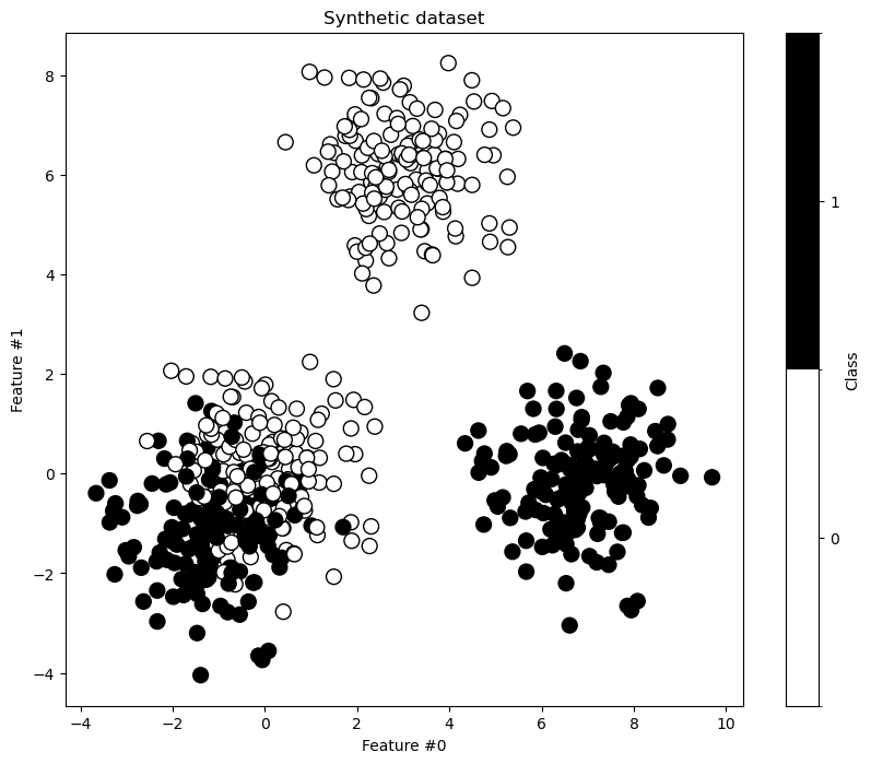
First, we train a shallow decision tree with max_depth=2. This depth should suffice to separate the easily separable blobs.
max_depth = 2
tree = DecisionTreeClassifier(max_depth=max_depth)
tree.fit(X, y)

_, ax = plt.subplots(figsize=(10, 8))
DecisionBoundaryDisplay.from_estimator(tree, X, cmap=plt.cm.RdBu, ax=ax)
data.plot.scatter(
    x="Feature #0",
    y="Feature #1",
    c="Class",
    s=100,
    edgecolor="black",
    ax=ax,
)
ax.set_title(f"Decision tree with max-depth of {max_depth}")
plt.show()
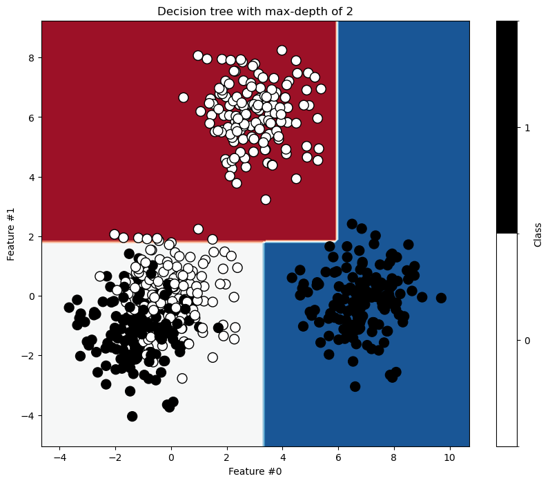
As expected, the blue blob on the right and red blob on top separate easily. However, we need more splits to better separate the mixed blobs.
The red blob on top and blue blob on the right separate perfectly. However, the tree still makes mistakes where the blobs mix. Let’s examine the tree structure.
_, ax = plt.subplots(figsize=(15, 8))
plot_tree(
    tree, feature_names=feature_names, class_names=class_names, filled=True, ax=ax
)
plt.show()
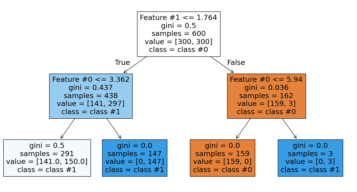
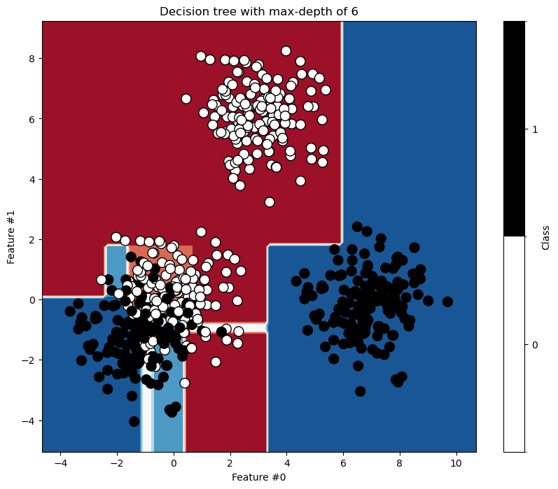
The right branch achieves perfect classification. Now we increase the depth to see how the tree grows.
max_depth = 6
tree = DecisionTreeClassifier(max_depth=max_depth)
tree.fit(X, y)
DecisionTreeClassifier(max_depth=6)In a Jupyter environment, please rerun this cell to show the HTML representation or trust the notebook.
On GitHub, the HTML representation is unable to render, please try loading this page with nbviewer.org.
DecisionTreeClassifier(max_depth=6)
_, ax = plt.subplots(figsize=(10, 8))
DecisionBoundaryDisplay.from_estimator(tree, X, cmap=plt.cm.RdBu, ax=ax)
data.plot.scatter(
    x="Feature #0",
    y="Feature #1",
    c="Class",
    s=100,
    edgecolor="black",
    ax=ax,
)
ax.set_title(f"Decision tree with max-depth of {max_depth}")
plt.show()
_, ax = plt.subplots(figsize=(25, 15))
plot_tree(
    tree, feature_names=feature_names, class_names=class_names, filled=True, ax=ax
)
plt.show()
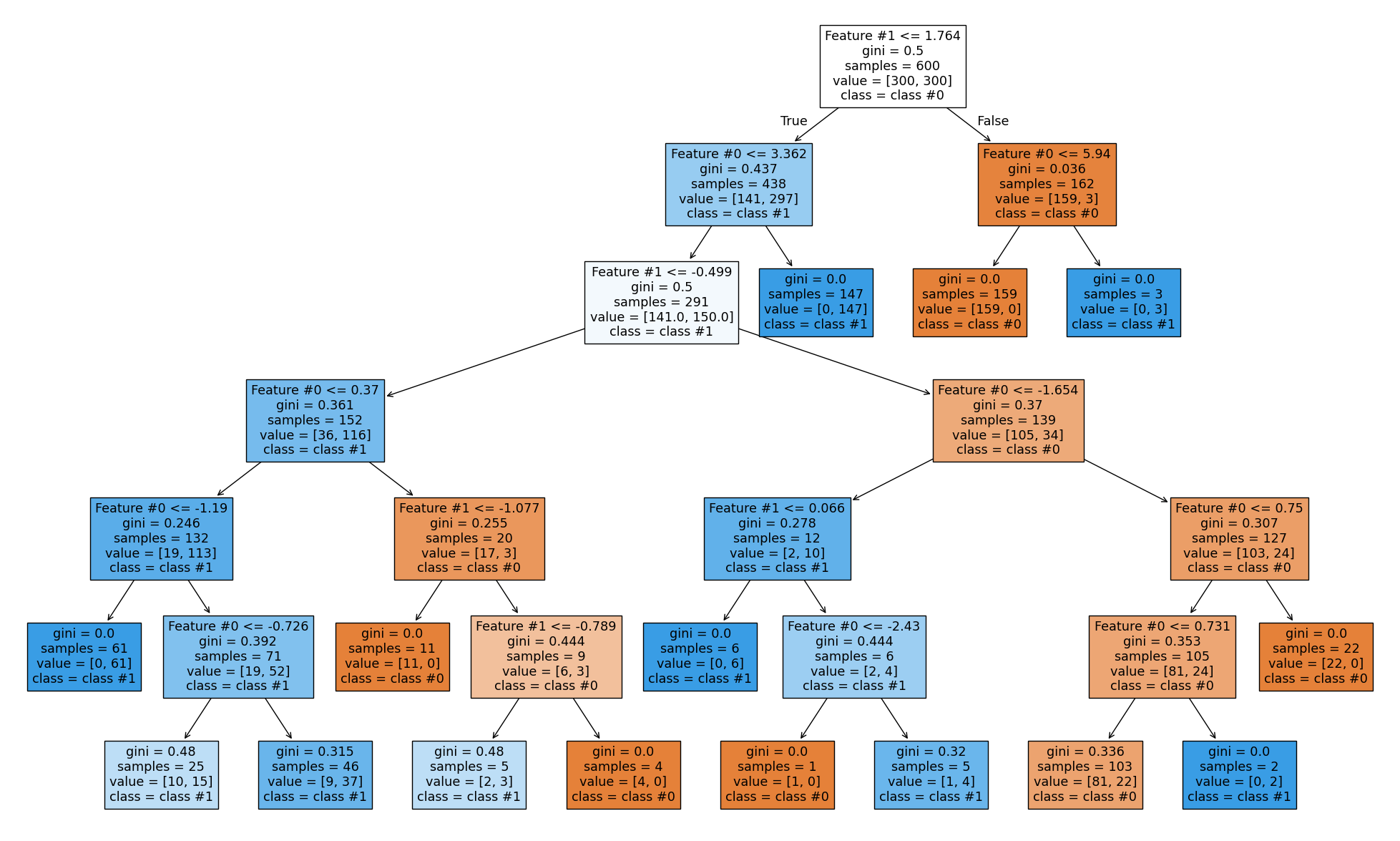
As expected, the left branch continues to grow while the right branch stops splitting. Setting max_depth cuts the tree horizontally at a specific level, whether or not a branch would benefit from growing further.
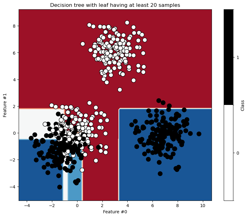
The hyperparameters min_samples_leaf, min_samples_split, max_leaf_nodes, and min_impurity_decrease allow asymmetric trees and apply constraints at the leaf or node level. Let’s examine the effect of min_samples_leaf.
min_samples_leaf = 20
tree = DecisionTreeClassifier(min_samples_leaf=min_samples_leaf)
tree.fit(X, y)

_, ax = plt.subplots(figsize=(10, 8))
DecisionBoundaryDisplay.from_estimator(tree, X, cmap=plt.cm.RdBu, ax=ax)
data.plot.scatter(
    x="Feature #0",
    y="Feature #1",
    c="Class",
    s=100,
    edgecolor="black",
    ax=ax,
)
ax.set_title(f"Decision tree with leaf having at least {min_samples_leaf} samples")
plt.show()
_, ax = plt.subplots(figsize=(15, 15))
plot_tree(
    tree, feature_names=feature_names, class_names=class_names, filled=True, ax=ax
)
plt.show()
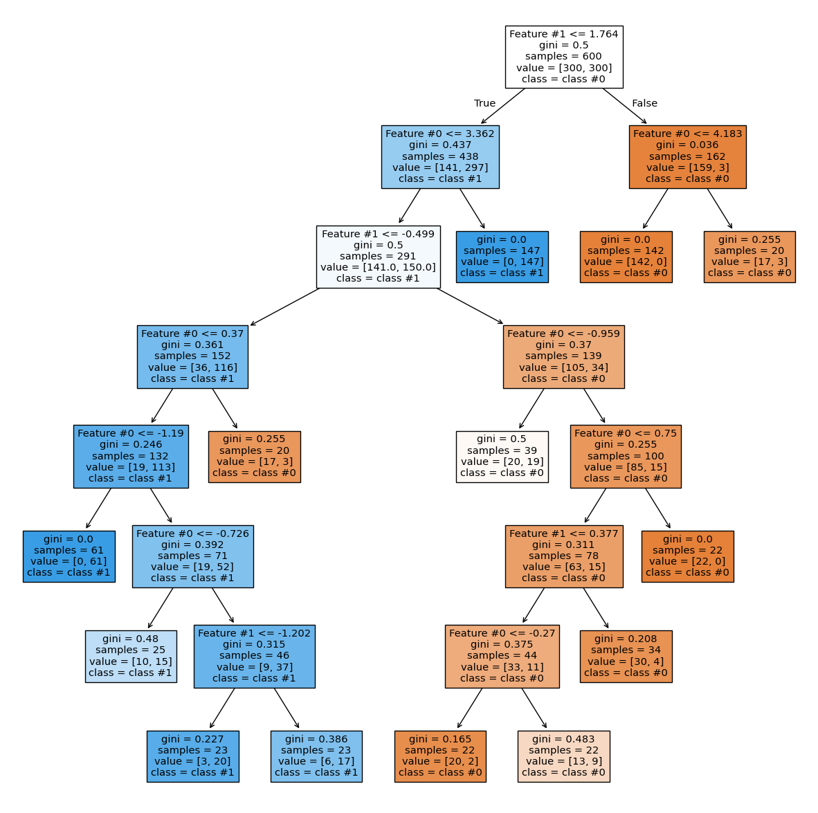
This hyperparameter ensures leaves contain a minimum number of samples and prevents further splits otherwise. These hyperparameters offer an alternative to the max_depth parameter.