Gaussian process

All models we have encountered so far provide a point-estimate during prediction. However, none of these models (except QuantileRegression) provide confidence intervals for their predictions.

Gaussian Process models allow us to obtain such information. In this notebook, we present how these models differ from the ones we already covered.

Let’s start by generating a toy dataset.

# When using JupyterLite, uncomment and install the `skrub` package.
%pip install skrub
import matplotlib.pyplot as plt
import skrub

skrub.patch_display()  # makes nice display for pandas tables

/home/runner/work/traces-sklearn/traces-sklearn/.pixi/envs/docs/bin/python: No module named pip

Note: you may need to restart the kernel to use updated packages.

import numpy as np

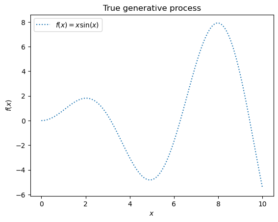
X = np.linspace(start=0, stop=10, num=1_000).reshape(-1, 1)
y = np.squeeze(X * np.sin(X))

_, ax = plt.subplots()
ax.plot(X, y, label=r"$f(x) = x \sin(x)$", linestyle="dotted")
ax.legend()
ax.set(xlabel="$x$", ylabel="$f(x)$", title="True generative process")
plt.show()

Example with noise-free target

In this first example, we use the true generative process without adding noise. For training the Gaussian Process regression, we select only a few samples.

rng = np.random.default_rng(1)
training_indices = rng.choice(np.arange(y.size), size=6, replace=False)
X_train, y_train = X[training_indices], y[training_indices]

A Gaussian kernel lets us craft a kernel by hand and compose base kernels together. Here, we use a radial basis function (RBF) kernel and a constant parameter to fit the amplitude.

from sklearn.gaussian_process import GaussianProcessRegressor
from sklearn.gaussian_process.kernels import RBF

kernel = 1 * RBF(length_scale=1.0, length_scale_bounds=(1e-2, 1e2))
gaussian_process = GaussianProcessRegressor(kernel=kernel, n_restarts_optimizer=20)

Previous methods we presented used a single model where we find optimal parameters that best fit the dataset. Gaussian Process uses a different paradigm: it works with a distribution of models. We start with a prior distribution of models. The training set combines with this prior to give us a posterior distribution of models.

First, let’s examine the prior distribution of our Gaussian process.

y_samples = gaussian_process.sample_y(X, n_samples=5)

_, ax = plt.subplots()
for idx, single_prior in enumerate(y_samples.T):
    ax.plot(
        X.ravel(),
        single_prior,
        linestyle="--",
        alpha=0.7,
        label=f"Sampled function #{idx + 1}",
    )

ax.legend(loc="center left", bbox_to_anchor=(1, 0.5))
ax.set(xlabel="$x$", ylabel="$f(x)$", title="Sample from the GP prior distribution")
plt.show()

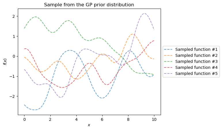
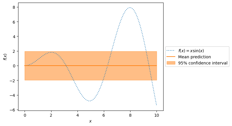
The samples from the prior distribution start as random realizations. They differ greatly from our true generative model. However, these samples form a distribution of models. We plot the mean and the 95% confidence interval.

mean_prediction, std_prediction = gaussian_process.predict(X, return_std=True)

_, ax = plt.subplots()
ax.plot(X, mean_prediction, label="Mean prediction")
ax.fill_between(
    X.ravel(),
    mean_prediction - 1.96 * std_prediction,
    mean_prediction + 1.96 * std_prediction,
    alpha=0.2,
    label=r"95% confidence interval",
    color="tab:blue",
)

for idx, single_prior in enumerate(y_samples.T):
    ax.plot(
        X.ravel(),
        single_prior,
        linestyle="--",
        alpha=0.7,
        label=f"Sampled function #{idx + 1}",
    )


ax.legend(loc="center left", bbox_to_anchor=(1, 0.5))
ax.set(
    xlabel="$x$", ylabel="$f(x)$", title="GP prediction using only prior distribution"
)
plt.show()

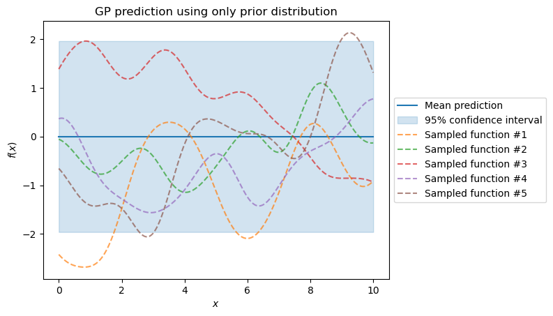
The true generative process and the prediction show we need to improve our model.

_, ax = plt.subplots()
ax.plot(X, y, label=r"$f(x) = x \sin(x)$", linestyle="dotted")
ax.plot(X, mean_prediction, label="Mean prediction")
ax.fill_between(
    X.ravel(),
    mean_prediction - 1.96 * std_prediction,
    mean_prediction + 1.96 * std_prediction,
    alpha=0.5,
    label=r"95% confidence interval",
    color="tab:orange",
)
ax.legend(loc="center left", bbox_to_anchor=(1, 0.5))
ax.set(xlabel="$x$", ylabel="$f(x)$")
plt.show()

Now, we fit a Gaussian process on these few training samples to see how they influence the posterior distribution.

gaussian_process.fit(X_train, y_train)
gaussian_process.kernel_

3.73**2 * RBF(length_scale=1.03)

After fitting our model, the hyperparameters of the kernel have been optimized. Now, we use our kernel to compute the mean prediction of the full dataset and plot the 95% confidence interval.

mean_prediction, std_prediction = gaussian_process.predict(X, return_std=True)

_, ax = plt.subplots()
ax.plot(X, y, label=r"$f(x) = x \sin(x)$", linestyle="dotted")
ax.scatter(X_train, y_train, label="Observations")
ax.plot(X, mean_prediction, label="Mean prediction")
ax.fill_between(
    X.ravel(),
    mean_prediction - 1.96 * std_prediction,
    mean_prediction + 1.96 * std_prediction,
    alpha=0.5,
    label=r"95% confidence interval",
)
ax.legend(loc="center left", bbox_to_anchor=(1, 0.5))
ax.set(
    xlabel="$x$",
    ylabel="$f(x)$",
    title="Gaussian process regression \non noise-free dataset",
)
plt.show()

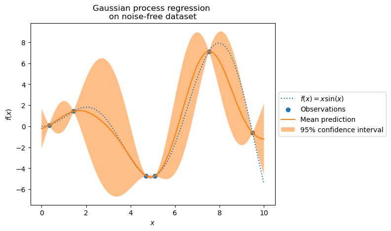
For predictions near training points, the 95% confidence interval shows small amplitude. When samples fall far from training data, our model predicts less accurately with higher uncertainty.

Example with noisy targets

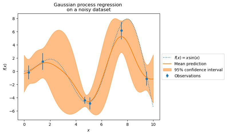
We repeat a similar experiment by adding noise to the target. This shows the effect of noise on the fitted model.

We add random Gaussian noise to the target with an arbitrary standard deviation.

dy = 0.5 + 1.0 * rng.uniform(size=y_train.shape)
y_train_noisy = y_train + rng.normal(0, dy)

We create a similar Gaussian process model. Along with the kernel, we specify the parameter alpha which represents the variance of Gaussian noise.

gaussian_process = GaussianProcessRegressor(
    kernel=kernel, alpha=dy**2, n_restarts_optimizer=9
)
gaussian_process.fit(X_train, y_train_noisy)
mean_prediction, std_prediction = gaussian_process.predict(X, return_std=True)

Let’s plot the mean prediction and uncertainty region.

_, ax = plt.subplots()
ax.plot(X, y, label=r"$f(x) = x \sin(x)$", linestyle="dotted")
ax.errorbar(
    X_train,
    y_train_noisy,
    dy,
    linestyle="None",
    color="tab:blue",
    marker=".",
    markersize=10,
    label="Observations",
)
ax.plot(X, mean_prediction, label="Mean prediction")
ax.fill_between(
    X.ravel(),
    mean_prediction - 1.96 * std_prediction,
    mean_prediction + 1.96 * std_prediction,
    color="tab:orange",
    alpha=0.5,
    label=r"95% confidence interval",
)
ax.legend(loc="center left", bbox_to_anchor=(1, 0.5))
ax.set(
    xlabel="$x$",
    ylabel="$f(x)$",
    title="Gaussian process regression \non a noisy dataset",
)
plt.show()

Exercise: Design a kernel for Gaussian Process

Build the dataset

The Mauna Loa Observatory collects air samples. We want to estimate the CO2 concentration and extrapolate it for future years. Let’s load the original dataset from OpenML.

# Uncomment this line in JupyterLite
%pip install pyodide-http
# import pyodide_http
# pyodide_http.patch_all()

/home/runner/work/traces-sklearn/traces-sklearn/.pixi/envs/docs/bin/python: No module named pip

Note: you may need to restart the kernel to use updated packages.

from sklearn.datasets import fetch_openml

co2 = fetch_openml(data_id=41187, as_frame=True)
co2.frame

Processing column   1 / 7

Processing column   2 / 7

Processing column   3 / 7

Processing column   4 / 7

Processing column   5 / 7

Processing column   6 / 7

Processing column   7 / 7

Please enable javascript

The skrub table reports need javascript to display correctly. If you are displaying a report in a Jupyter notebook and you see this message, you may need to re-execute the cell or to trust the notebook (button on the top right or "File > Trust notebook").

First, we create a date index and select only the CO2 column.

import pandas as pd

co2_data = co2.frame
co2_data["date"] = pd.to_datetime(co2_data[["year", "month", "day"]])
co2_data = co2_data[["date", "co2"]].set_index("date")
co2_data

Processing column   1 / 1

Please enable javascript

The skrub table reports need javascript to display correctly. If you are displaying a report in a Jupyter notebook and you see this message, you may need to re-execute the cell or to trust the notebook (button on the top right or "File > Trust notebook").

co2_data.index.min(), co2_data.index.max()

(Timestamp('1958-03-29 00:00:00'), Timestamp('2001-12-29 00:00:00'))

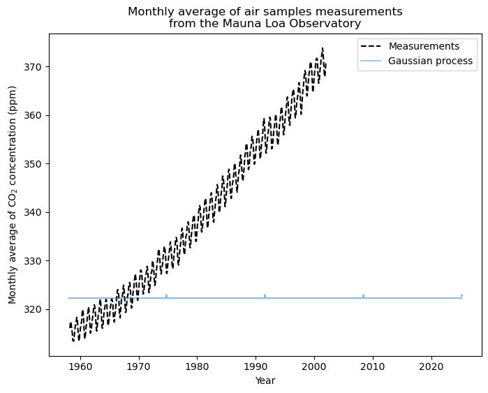
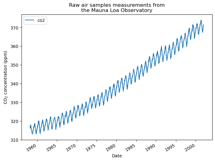
The data shows CO2 concentration measurements from March 1958 to December 2001. Let’s plot this raw information.

_, ax = plt.subplots(figsize=(8, 6))
co2_data.plot(ax=ax)
ax.set(
    xlabel="Date",
    ylabel="CO$_2$ concentration (ppm)",
    title="Raw air samples measurements from\nthe Mauna Loa Observatory",
)
plt.show()

We take a monthly average and drop months without measurements. This smooths the data.

_, ax = plt.subplots(figsize=(8, 6))
co2_data = co2_data.resample("ME").mean().dropna(axis="index", how="any")
co2_data.plot(ax=ax)
ax.set(
    ylabel="Monthly average of CO$_2$ concentration (ppm)",
    title=(
        "Monthly average of air samples measurements\n from the Mauna Loa Observatory",
    ),
)
plt.show()

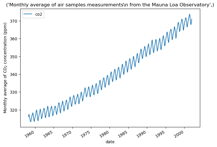
We want to predict the CO2 concentration based on the date. We also want to extrapolate values for years after 2001.

First, we split the data and target. We convert the dates into numeric values.

X_train = (co2_data.index.year + co2_data.index.month / 12).to_numpy().reshape(-1, 1)
y_train = co2_data["co2"].to_numpy()

Exercise

Let’s repeat the experiment from [1] (Sect. 5.4.3, p.119-122) by designing a handmade kernel.

Let’s recall the definition of the kernel. The long-term trend is modeled by a squared exponential kernel.

\[ k_{1}(x, x') = \theta_{1}^2 \exp\left( -\frac{(x - x')^2}{2 \theta_{2}^2} \right) \]

The seasonal component uses an exponential sine squared kernel to encode the periodicity. However, since the signal is not exactly periodic, it is fixed by multiplying by a squared exponential kernel. Thus, it is defined as:

\[ k_{2}(x, x') = \theta_{3}^2 \exp\left( -\frac{(x - x')^2}{2 \theta_{4}^2} - \frac{2 \sin^2\left(\pi (x - x') \right)}{\theta_{5}^2} \right) \]

The irregularities are modeled by a rational quadratic kernel.

\[ k_{3}(x, x') = \theta_{6}^2 \left( 1 + \frac{(x - x')^2}{2 \theta_{8} \theta_{7}^2} \right)^{-\theta_{8}} \]

Finally, we add a noise component to the kernel that is modeled by a squared exponential kernel.

\[ k_{4}(x, x') = \theta_{9}^2 \exp\left( -\frac{(x - x')^2}{2 \theta_{10}^2} \right) + \theta_{11}^2 \delta_{x, x'} \]

The final kernel is a sum of the previous kernels:

\[ k(x, x') = \theta_0 + k_{1}(x, x') + k_{2}(x, x') + k_{3}(x, x') + k_{4}(x, x') \]

Where \(\theta_0\) is a constant offset equal to the mean of the target.

References:

[1] Rasmussen, C. E., & Williams, C. K. (2006). Gaussian Processes for Machine Learning. The MIT Press. https://gaussianprocess.org/gpml/chapters/RW.pdf

Let’s provide the bare-bones code to fit a Gaussian process with this kernel.

import datetime
import numpy as np

today = datetime.datetime.now()
current_month = today.year + today.month / 12
X_test = np.linspace(start=1958, stop=current_month, num=1_000).reshape(-1, 1)

from sklearn.gaussian_process.kernels import (
    ConstantKernel,
    ExpSineSquared,  # noqa: F401
    RationalQuadratic,  # noqa: F401
    WhiteKernel,  # noqa: F401
)

constant_kernel = ConstantKernel(constant_value=y_train.mean())
long_term_trend_kernel = 1.0**2
seasonal_kernel = 1.0**2
irregularities_kernel = 1.0**2
noise_kernel = 1.0**2

co2_kernel = (
    constant_kernel
    + long_term_trend_kernel
    + seasonal_kernel
    + irregularities_kernel
    + noise_kernel
)

gaussian_process = GaussianProcessRegressor(
    kernel=co2_kernel, normalize_y=False, n_restarts_optimizer=1
)
gaussian_process.fit(X_train, y_train)
mean_y_pred, std_y_pred = gaussian_process.predict(X_test, return_std=True)

/home/runner/work/traces-sklearn/traces-sklearn/.pixi/envs/docs/lib/python3.12/site-packages/sklearn/gaussian_process/kernels.py:442: ConvergenceWarning: The optimal value found for dimension 0 of parameter k1__k1__k1__k1__constant_value is close to the specified lower bound 1e-05. Decreasing the bound and calling fit again may find a better value.
  warnings.warn(
/home/runner/work/traces-sklearn/traces-sklearn/.pixi/envs/docs/lib/python3.12/site-packages/sklearn/gaussian_process/kernels.py:442: ConvergenceWarning: The optimal value found for dimension 0 of parameter k1__k1__k1__k2__constant_value is close to the specified lower bound 1e-05. Decreasing the bound and calling fit again may find a better value.
  warnings.warn(
/home/runner/work/traces-sklearn/traces-sklearn/.pixi/envs/docs/lib/python3.12/site-packages/sklearn/gaussian_process/kernels.py:442: ConvergenceWarning: The optimal value found for dimension 0 of parameter k1__k1__k2__constant_value is close to the specified lower bound 1e-05. Decreasing the bound and calling fit again may find a better value.
  warnings.warn(
/home/runner/work/traces-sklearn/traces-sklearn/.pixi/envs/docs/lib/python3.12/site-packages/sklearn/gaussian_process/kernels.py:452: ConvergenceWarning: The optimal value found for dimension 0 of parameter k1__k2__constant_value is close to the specified upper bound 100000.0. Increasing the bound and calling fit again may find a better value.
  warnings.warn(
/home/runner/work/traces-sklearn/traces-sklearn/.pixi/envs/docs/lib/python3.12/site-packages/sklearn/gaussian_process/kernels.py:442: ConvergenceWarning: The optimal value found for dimension 0 of parameter k2__constant_value is close to the specified lower bound 1e-05. Decreasing the bound and calling fit again may find a better value.
  warnings.warn(
/home/runner/work/traces-sklearn/traces-sklearn/.pixi/envs/docs/lib/python3.12/site-packages/sklearn/gaussian_process/_gpr.py:477: UserWarning: Predicted variances smaller than 0. Setting those variances to 0.
  warnings.warn(

_, ax = plt.subplots(figsize=(8, 6))
ax.plot(X_train, y_train, color="black", linestyle="dashed", label="Measurements")
ax.plot(X_test, mean_y_pred, color="tab:blue", alpha=0.4, label="Gaussian process")
ax.fill_between(
    X_test.ravel(),
    mean_y_pred - std_y_pred,
    mean_y_pred + std_y_pred,
    color="tab:blue",
    alpha=0.2,
)
ax.legend()
ax.set_xlabel("Year")
ax.set_ylabel("Monthly average of CO$_2$ concentration (ppm)")
_ = ax.set_title(
    "Monthly average of air samples measurements\n" "from the Mauna Loa Observatory"
)