Bagged trees

# When using JupyterLite, uncomment and install the `skrub` package.
%pip install skrub
import matplotlib.pyplot as plt
import skrub

skrub.patch_display()  # makes nice display for pandas tables

/home/runner/work/traces-sklearn/traces-sklearn/.pixi/envs/docs/bin/python: No module named pip

Note: you may need to restart the kernel to use updated packages.

Bagging estimator

We see that increasing the depth of the tree leads to an over-fitted model. We can bypass choosing a specific depth by combining several trees together.

Let’s start by training several trees on slightly different data. We can generate slightly different datasets by randomly sampling with replacement. In statistics, we call this a bootstrap sample. We will use the iris dataset to create such an ensemble and keep some data for training and testing.

from sklearn.datasets import load_iris
from sklearn.model_selection import train_test_split

X, y = load_iris(return_X_y=True)
X, y = X[:100], y[:100]
X_train, X_test, y_train, y_test = train_test_split(X, y, stratify=y)

Before training several decision trees, let’s run a single tree. Instead of training this tree on X_train, we want to train it on a bootstrap sample. We can use the np.random.choice function to sample indices with replacement. We need to create a sample_weight vector and pass it to the fit method of the DecisionTreeClassifier. We provide the generate_sample_weight function to generate the sample_weight array.

import numpy as np


def bootstrap_idx(X):
    indices = np.random.choice(np.arange(X.shape[0]), size=X.shape[0], replace=True)
    return indices

bootstrap_idx(X_train)

array([ 5, 30, 56, 17, 65,  8, 72, 14, 25, 21, 50, 70, 50, 59, 68, 65, 28,
       36, 15, 30, 14, 60, 54, 27, 40, 23, 61, 39,  9,  5,  4, 26,  5, 56,
       52, 18, 15, 62, 56,  2, 38, 64, 67, 64, 47,  9, 65, 58, 60, 20, 11,
       40, 60,  3,  5,  3,  9, 34, 29, 72, 37, 14, 14, 28, 61, 73,  6, 58,
        1,  7, 28, 20, 47, 60, 34])

from collections import Counter

Counter(bootstrap_idx(X_train))

Counter({np.int64(66): 3,
         np.int64(29): 3,
         np.int64(10): 3,
         np.int64(71): 3,
         np.int64(44): 3,
         np.int64(65): 2,
         np.int64(4): 2,
         np.int64(34): 2,
         np.int64(46): 2,
         np.int64(55): 2,
         np.int64(61): 2,
         np.int64(39): 2,
         np.int64(68): 2,
         np.int64(24): 2,
         np.int64(5): 2,
         np.int64(9): 2,
         np.int64(43): 2,
         np.int64(3): 2,
         np.int64(15): 2,
         np.int64(67): 2,
         np.int64(56): 2,
         np.int64(53): 2,
         np.int64(59): 1,
         np.int64(52): 1,
         np.int64(16): 1,
         np.int64(74): 1,
         np.int64(69): 1,
         np.int64(11): 1,
         np.int64(33): 1,
         np.int64(41): 1,
         np.int64(28): 1,
         np.int64(63): 1,
         np.int64(7): 1,
         np.int64(0): 1,
         np.int64(1): 1,
         np.int64(12): 1,
         np.int64(20): 1,
         np.int64(13): 1,
         np.int64(60): 1,
         np.int64(27): 1,
         np.int64(72): 1,
         np.int64(50): 1,
         np.int64(8): 1,
         np.int64(38): 1,
         np.int64(54): 1,
         np.int64(32): 1,
         np.int64(73): 1,
         np.int64(14): 1})

def bootstrap_sample(X, y):
    indices = bootstrap_idx(X)
    return X[indices], y[indices]

X_train_bootstrap, y_train_bootstrap = bootstrap_sample(X_train, y_train)

print(f"Classes distribution in the original data: {Counter(y_train)}")
print(f"Classes distribution in the bootstrap: {Counter(y_train_bootstrap)}")

Classes distribution in the original data: Counter({np.int64(0): 38, np.int64(1): 37})
Classes distribution in the bootstrap: Counter({np.int64(1): 46, np.int64(0): 29})

EXERCISE: Create a bagging classifier

A bagging classifier trains several decision tree classifiers, each on a different bootstrap sample.

1. Create several DecisionTreeClassifier instances and store them in a Python list

2. Loop through these trees and fit them by generating a bootstrap sample using the bootstrap_sample function

3. To predict with this ensemble on new data (testing set), provide the same set to each tree and call the predict method. Aggregate all predictions in a NumPy array

4. Once you have the predictions, provide a single prediction by keeping the most predicted class (majority vote)

5. Check the accuracy of your model

# Write your code here.

EXERCISE: Using scikit-learn

After implementing your own bagging classifier, use scikit-learn’s BaggingClassifier to fit the above data.

# Write your code here.

Note about the base estimator

In the previous section, we used a decision tree as the base estimator in the bagging ensemble. However, this method accepts any kind of base estimator. We will compare two bagging models: one uses decision trees and another uses a linear model with a preprocessing step.

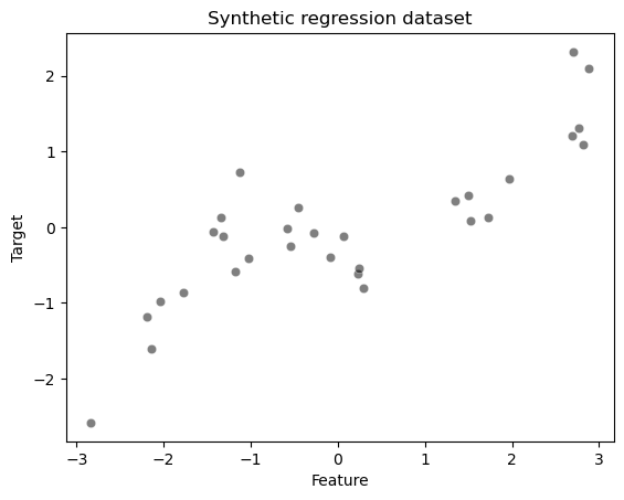
Let’s first create a synthetic regression dataset.

import pandas as pd

# Create a random number generator to set the randomness
rng = np.random.default_rng(1)

n_samples = 30
x_min, x_max = -3, 3
x = rng.uniform(x_min, x_max, size=n_samples)
noise = 4.0 * rng.normal(size=n_samples)
y = x**3 - 0.5 * (x + 1) ** 2 + noise
y /= y.std()

data_train = pd.DataFrame(x, columns=["Feature"])
data_test = pd.DataFrame(np.linspace(x_max, x_min, num=300), columns=["Feature"])
target_train = pd.Series(y, name="Target")

# Uncomment this line in JupyterLite
%pip install seaborn
import seaborn as sns

ax = sns.scatterplot(x=data_train["Feature"], y=target_train, color="black", alpha=0.5)
ax.set_title("Synthetic regression dataset")
plt.show()

/home/runner/work/traces-sklearn/traces-sklearn/.pixi/envs/docs/bin/python: No module named pip

Note: you may need to restart the kernel to use updated packages.

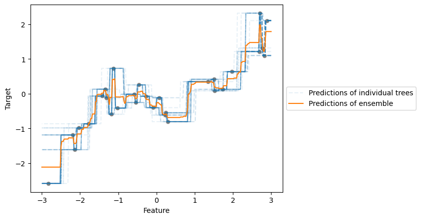
We will first train a BaggingRegressor where the base estimators are DecisionTreeRegressor instances.

from sklearn.ensemble import BaggingRegressor

bagged_trees = BaggingRegressor(n_estimators=50, random_state=0)
bagged_trees.fit(data_train, target_train)

BaggingRegressor(n_estimators=50, random_state=0)

In a Jupyter environment, please rerun this cell to show the HTML representation or trust the notebook.
On GitHub, the HTML representation is unable to render, please try loading this page with nbviewer.org.

We can make a plot showing the prediction from each individual tree and the averaged response from the bagging regressor.

for tree_idx, tree in enumerate(bagged_trees.estimators_):
    label = "Predictions of individual trees" if tree_idx == 0 else None
    tree_predictions = tree.predict(data_test.to_numpy())
    plt.plot(
        data_test,
        tree_predictions,
        linestyle="--",
        alpha=0.1,
        color="tab:blue",
        label=label,
    )

sns.scatterplot(x=data_train["Feature"], y=target_train, color="black", alpha=0.5)

bagged_trees_predictions = bagged_trees.predict(data_test)
plt.plot(
    data_test,
    bagged_trees_predictions,
    color="tab:orange",
    label="Predictions of ensemble",
)
plt.legend(loc="center left", bbox_to_anchor=(1, 0.5))
plt.show()

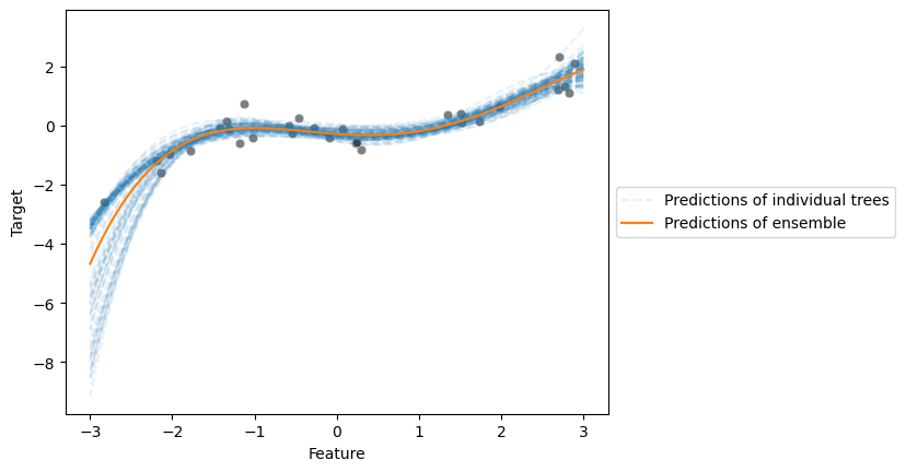
Now, we will show that we can use a model other than a decision tree. We will create a model that uses PolynomialFeatures to augment features followed by a Ridge linear model.

from sklearn.linear_model import Ridge
from sklearn.pipeline import make_pipeline
from sklearn.preprocessing import MinMaxScaler, PolynomialFeatures

polynomial_regressor = make_pipeline(
    MinMaxScaler(),
    PolynomialFeatures(degree=4),
    Ridge(alpha=1e-10),
)

bagged_trees = BaggingRegressor(
    n_estimators=100, estimator=polynomial_regressor, random_state=0
)
bagged_trees.fit(data_train, target_train)

for tree_idx, tree in enumerate(bagged_trees.estimators_):
    label = "Predictions of individual trees" if tree_idx == 0 else None
    tree_predictions = tree.predict(data_test.to_numpy())
    plt.plot(
        data_test,
        tree_predictions,
        linestyle="--",
        alpha=0.1,
        color="tab:blue",
        label=label,
    )

sns.scatterplot(x=data_train["Feature"], y=target_train, color="black", alpha=0.5)

bagged_trees_predictions = bagged_trees.predict(data_test)
plt.plot(
    data_test,
    bagged_trees_predictions,
    color="tab:orange",
    label="Predictions of ensemble",
)
plt.legend(loc="center left", bbox_to_anchor=(1, 0.5))
plt.show()

We observe that both base estimators can model our toy example effectively.

Random Forests

Random forest classifier

The random forest classifier is a popular variant of the bagging classifier. In addition to bootstrap sampling, random forest uses a random subset of features to find the best split.

EXERCISE: Create a random forest classifier

Use your previous code that generated several DecisionTreeClassifier instances. Check the classifier options and modify the parameters to use only \(\sqrt{F}\) features for splitting, where \(F\) represents the number of features in the dataset.

# Write your code here.

EXERCISE: Using scikit-learn

After implementing your own random forest classifier, use scikit-learn’s RandomForestClassifier to fit the above data.

# Write your code here.

Random forest regressor

EXERCISE:

1. Load the dataset from sklearn.datasets.fetch_california_housing

2. Fit a RandomForestRegressor with default parameters

3. Find the number of features used during training

4. Identify the differences between BaggingRegressor and RandomForestRegressor

# Write your code here.

Hyperparameters

The hyperparameters affecting the training process match those of decision trees. Check the documentation for details. Since we work with a forest of trees, we have an additional parameter n_estimators. Let’s examine how this parameter affects performance using a validation curve.

# Uncomment this line in JupyterLite
%pip install pyodide-http
# import pyodide_http
# pyodide_http.patch_all()

/home/runner/work/traces-sklearn/traces-sklearn/.pixi/envs/docs/bin/python: No module named pip

Note: you may need to restart the kernel to use updated packages.

from sklearn.datasets import fetch_california_housing

X, y = fetch_california_housing(return_X_y=True, as_frame=True)

EXERCISE:

1. Compute train and test scores to analyze how the n_estimators parameter affects performance. Define a range of values for this parameter

2. Plot the train and test scores with confidence intervals

Consider: How does increasing the number of trees affect statistical performance? What trade-offs exist with computational performance?

# Write your code here.

You can also tune other parameters that control individual tree overfitting. Sometimes shallow trees suffice. However, random forests typically use deep trees since we want to overfit the learners on bootstrap samples - the ensemble combination mitigates this overfitting. Using shallow (underfitted) trees may lead to an underfitted forest.