Quantile regression#
This notebook explores how to predict intervals with available techniques in scikit-learn.
We cover a subset of available techniques. For instance, conformal predictions handle this specific task - see packages like MAPIE for broader coverage: scikit-learn-contrib/MAPIE.
Predicting intervals with linear models#
This section revisits linear models and shows how to predict intervals with quantile regression.
First, let’s load our penguins dataset for our regression task.
# When using JupyterLite, uncomment and install the `skrub` package.
%pip install skrub
import matplotlib.pyplot as plt
import skrub

skrub.patch_display()
/home/runner/work/traces-sklearn/traces-sklearn/.pixi/envs/docs/bin/python: No module named pip
Note: you may need to restart the kernel to use updated packages.
import pandas as pd

penguins = pd.read_csv("../datasets/penguins_regression.csv")
penguins
Processing column 1 / 2
Processing column 2 / 2
| Flipper Length (mm) | Body Mass (g) | |
|---|---|---|
| 0 | 181.0 | 3750.0 |
| 1 | 186.0 | 3800.0 |
| 2 | 195.0 | 3250.0 |
| 3 | 193.0 | 3450.0 |
| 4 | 190.0 | 3650.0 |
| 337 | 207.0 | 4000.0 |
| 338 | 202.0 | 3400.0 |
| 339 | 193.0 | 3775.0 |
| 340 | 210.0 | 4100.0 |
| 341 | 198.0 | 3775.0 |
Flipper Length (mm)
Float64DType- Null values
- 0 (0.0%)
- Unique values
- 55 (16.1%)
- Mean ± Std
- 201. ± 14.1
- Median ± IQR
- 197. ± 23.0
- Min | Max
- 172. | 231.
Body Mass (g)
Float64DType- Null values
- 0 (0.0%)
- Unique values
- 94 (27.5%)
- Mean ± Std
- 4.20e+03 ± 802.
- Median ± IQR
- 4.05e+03 ± 1.20e+03
- Min | Max
- 2.70e+03 | 6.30e+03
No columns match the selected filter: . You can change the column filter in the dropdown menu above.
| Column | Column name | dtype | Null values | Unique values | Mean | Std | Min | Median | Max |
|---|---|---|---|---|---|---|---|---|---|
| 0 | Flipper Length (mm) | Float64DType | 0 (0.0%) | 55 (16.1%) | 201. | 14.1 | 172. | 197. | 231. |
| 1 | Body Mass (g) | Float64DType | 0 (0.0%) | 94 (27.5%) | 4.20e+03 | 802. | 2.70e+03 | 4.05e+03 | 6.30e+03 |
No columns match the selected filter: . You can change the column filter in the dropdown menu above.
Flipper Length (mm)
Float64DType- Null values
- 0 (0.0%)
- Unique values
- 55 (16.1%)
- Mean ± Std
- 201. ± 14.1
- Median ± IQR
- 197. ± 23.0
- Min | Max
- 172. | 231.
Body Mass (g)
Float64DType- Null values
- 0 (0.0%)
- Unique values
- 94 (27.5%)
- Mean ± Std
- 4.20e+03 ± 802.
- Median ± IQR
- 4.05e+03 ± 1.20e+03
- Min | Max
- 2.70e+03 | 6.30e+03
No columns match the selected filter: . You can change the column filter in the dropdown menu above.
| Column 1 | Column 2 | Cramér's V |
|---|---|---|
| Flipper Length (mm) | Body Mass (g) | 0.421 |
Please enable javascript
The skrub table reports need javascript to display correctly. If you are displaying a report in a Jupyter notebook and you see this message, you may need to re-execute the cell or to trust the notebook (button on the top right or "File > Trust notebook").
In this dataset, we predict the body mass of a penguin given its flipper length.
X = penguins[["Flipper Length (mm)"]]
y = penguins["Body Mass (g)"]
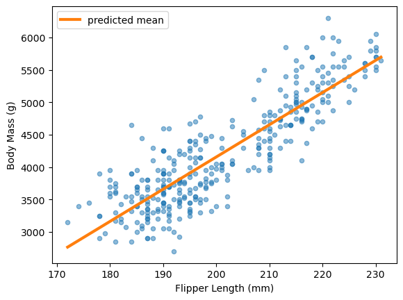
In our study of linear models, we saw that LinearRegression minimizes the mean
squared error and predicts the conditional mean of the target.
Here, we fit this model and predict several data points between the minimum and maximum flipper length.
from sklearn.linear_model import LinearRegression

model_estimate_mean = LinearRegression()
model_estimate_mean.fit(X, y)
LinearRegression()In a Jupyter environment, please rerun this cell to show the HTML representation or trust the notebook.
On GitHub, the HTML representation is unable to render, please try loading this page with nbviewer.org.
LinearRegression()
import numpy as np

X_test = pd.DataFrame(
    {"Flipper Length (mm)": np.linspace(X.min(axis=None), X.max(axis=None), 100)}
)
y_pred_mean = model_estimate_mean.predict(X_test)
_, ax = plt.subplots()
penguins.plot.scatter(x="Flipper Length (mm)", y="Body Mass (g)", ax=ax, alpha=0.5)
ax.plot(
    X_test["Flipper Length (mm)"],
    y_pred_mean,
    color="tab:orange",
    label="predicted mean",
    linewidth=3,
)
ax.legend()
plt.show()

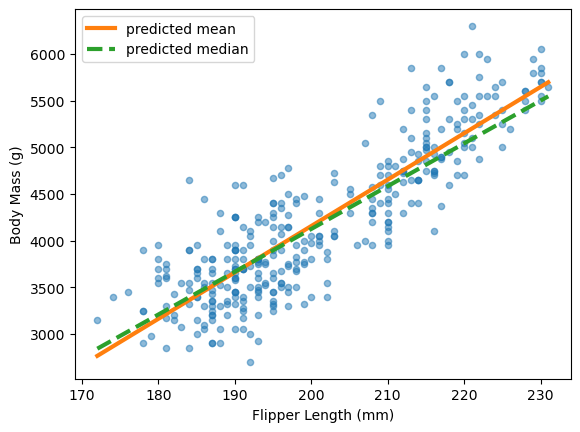
We discussed how mean estimators become sensitive to outliers. Sometimes we prefer a more robust estimator like the median.
Here, QuantileRegressor minimizes the mean absolute error and predicts the
conditional median.
from sklearn.linear_model import QuantileRegressor

model_estimate_median = QuantileRegressor(quantile=0.5)
model_estimate_median.fit(X, y)
y_pred_median = model_estimate_median.predict(X_test)
_, ax = plt.subplots()
penguins.plot.scatter(x="Flipper Length (mm)", y="Body Mass (g)", ax=ax, alpha=0.5)
ax.plot(
    X_test["Flipper Length (mm)"],
    y_pred_mean,
    color="tab:orange",
    label="predicted mean",
    linewidth=3,
)
ax.plot(
    X_test["Flipper Length (mm)"],
    y_pred_median,
    color="tab:green",
    label="predicted median",
    linewidth=3,
    linestyle="--",
)
ax.legend()
plt.show()

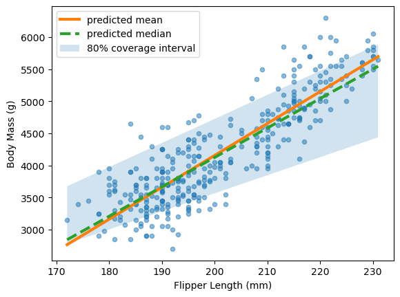
For confidence intervals, we want to predict specific quantiles. We generalize quantile regression beyond the median. The pinball loss generalizes the mean absolute error for any quantile.
The quantile parameter sets which quantile to predict. For an 80% prediction
interval, we predict the 10th and 90th percentiles.
model_estimate_10 = QuantileRegressor(quantile=0.1)
model_estimate_90 = QuantileRegressor(quantile=0.9)

model_estimate_10.fit(X, y)
model_estimate_90.fit(X, y)

y_pred_10 = model_estimate_10.predict(X_test)
y_pred_90 = model_estimate_90.predict(X_test)
_, ax = plt.subplots()
penguins.plot.scatter(x="Flipper Length (mm)", y="Body Mass (g)", ax=ax, alpha=0.5)
ax.plot(
    X_test["Flipper Length (mm)"],
    y_pred_mean,
    color="tab:orange",
    label="predicted mean",
    linewidth=3,
)
ax.plot(
    X_test["Flipper Length (mm)"],
    y_pred_median,
    color="tab:green",
    label="predicted median",
    linewidth=3,
    linestyle="--",
)
ax.fill_between(
    X_test["Flipper Length (mm)"],
    y_pred_10,
    y_pred_90,
    alpha=0.2,
    label="80% coverage interval",
)
ax.legend()
plt.show()

Predicting intervals with tree-based models#
Exercise:
Now repeat the previous experiment using HistGradientBoostingRegressor. Read
the documentation to find the parameters that optimize the right loss function.
Plot the conditional mean, median and 80% prediction interval.
# Write your code here.